Introducing causal discovery to PyMC-Marketing

In marketing, we love to tell stories about what drives what: “TV lifts organic traffic,” “Meta drives sign-ups,” “price cuts increase search volume.” Yet those stories rely on an unspoken assumption — that we actually know the direction of influence. What if the “driver” is really a downstream effect of something else, like seasonality or product launches? Without a causal map, even elegant regressions or Bayesian models can mistake correlation for causation, leading us to optimize the wrong levers.

That’s where causal discovery enters: algorithms that learn the underlying graph of cause and effect by testing conditional independences in data. The classical PC and FCI algorithms, used in fields like biology and neuroscience, are brilliant at uncovering causal skeletons under strong assumptions — i.i.d. data, no feedback, and well-separated mechanisms. But marketing rarely plays by those rules. Channels interact, campaigns overlap in time, and KPIs often feed back into exposure decisions. The result? Run a vanilla PC or FCI on raw marketing data, and you’ll likely get nonsense: edges pointing from conversions to impressions, from CTR to spend, or loops that defy business logic.

Does this mean causal discovery is hopeless for marketing? Not at all. Marketing systems are structural, not chaotic. We already know many relationships cannot exist — impressions don’t depend on conversions, and every causal path should eventually point toward a measurable target or KPI. We also have strong priors about latent factors like seasonality or market share dynamics. This knowledge drastically reduces the search space and makes causal discovery feasible if we incorporate it thoughtfully. That’s exactly what this notebook explores.

TBFPC algorithm overview

The TBFPC algorithm — Target-first Bayes Factor PC — is a lightweight, target-oriented variant of the classical PC approach, designed with marketing in mind. It tests for independence using Bayes factors instead of frequentist tests, and lets you encode forbidden edges to reflect domain priors. It adds a target-edge rule — "any", "conservative", or "fullS" — to bias discovery toward genuine driver → target relationships. The Bayes factor is computed via the ΔBIC approximation:

TBFPC is experimental, but it bridges an important gap between Bayesian modeling and causal reasoning for marketing science. It aims not to replace classical discovery frameworks, but to adapt them — respecting the structure, constraints, and realities of marketing data — to yield graphs that make sense both statistically and strategically.

Glossary

1. Causal discovery – Algorithms that infer directional relationships between variables by testing conditional independences in observational data.

2. Directed Acyclic Graph (DAG) – A fully oriented, cycle-free graph that encodes one specific causal data-generating process.

3. Completed Partially Directed Acyclic Graph (CPDAG) – A graph with both directed and undirected edges summarizing every DAG in the same Markov equivalence class.

4. Markov equivalence class (MEC) – The collection of DAGs that imply identical d-separation statements and therefore cannot be distinguished via conditional independence tests alone.

5. Target-first Bayes Factor PC (TBFPC) – Target-oriented adaptation of the PC discovery algorithm that applies Bayes factor (ΔBIC) tests plus marketing-specific constraints to learn causal skeletons.

6. Bayes factor ΔBIC test – The log Bayes factor computed from the change in Bayesian Information Criterion, used to decide whether variables remain dependent after conditioning on controls.

Import dependencies

# avoid all warnings types
import warnings

warnings.filterwarnings("ignore")

import os
import tempfile

import arviz as az
import matplotlib.image as mpimg
import matplotlib.pyplot as plt
import numpy as np
import pandas as pd
import preliz as pz
import pymc as pm
from graphviz import Digraph, Source
from IPython.display import SVG, display

from pymc_marketing.causal_utils import same_markov_equivalence_class_CPdag
from pymc_marketing.mmm.causal import (
    TBFPC,
    BuildModelFromDAG,
)

OMP: Info #276: omp_set_nested routine deprecated, please use omp_set_max_active_levels instead.

Setting notebook

az.style.use("arviz-darkgrid")
plt.rcParams["figure.figsize"] = [12, 7]
plt.rcParams["figure.dpi"] = 200
plt.rcParams.update({"figure.constrained_layout.use": True})

%load_ext autoreload
%autoreload 2
%config InlineBackend.figure_format = "retina"

seed = sum(map(ord, "Causality and Bayes as you never saw it before"))
rng = np.random.default_rng(seed)
n_observations = 1050

Let’s begin with a simple but powerful causal story, adapted from an article by Ben Vincent — “Causal Inference: have you been doing science wrong all this time?”. In it, Ben illustrates (probably without know it) a common situation in marketing analytics where search, media, and sales are tightly interwoven. We’ll recreate a similar structure here, representing the true (but usually hidden) causal data-generating process.

Imagine the following system:

• People first engage with generic search activity (Q), such as looking for products or comparing options.

• This general intent influences media exposure (X) — those who are searching more are also more likely to see or click ads.

• Both Q and X shape brand search (Y), which captures the strength of the brand in the customer’s mind.

• Finally, both X and Y lead to purchases (P).

This graph tells a clear causal story: upstream intent (Q) drives both media and brand search, which together drive sales. Yet, if we didn’t know this map and simply ran a regression of P ~ X + Y, we might overestimate the effect of X (media) because part of its variation is confounded by Q. Or we might mistakenly interpret Y (brand search) as an independent driver of purchases, when in reality it is mediated by media and intent. This is the classic trap of confusing correlation with causation.

Such structures are not hypothetical — they mirror real marketing dynamics. Channels, brand signals, and consumer intent often reinforce each other. Without a causal understanding of how these processes interact, any econometric or Bayesian model risks attributing the wrong effects to the wrong levers. Causal discovery gives us a principled way to uncover (or at least approximate) this hidden DAG, helping us build models that explain why something happens — not just what happens. The next cell visualizes this canonical causal map.

# Define the true DAG structure for our synthetic data
true_dag = Digraph(comment="True Causal DAG")
true_dag.attr(rankdir="LR")
true_dag.node("Q", "generic_search")
true_dag.node("X", "media_activities")
true_dag.node("Y", "brand_search")
true_dag.node("P", "purchase", fillcolor="lightgrey", style="filled")

# edges
true_dag.edge("Q", "X")  # Q influences X
true_dag.edge("Q", "Y")  # Q influences Y
true_dag.edge("X", "Y")  # X influences Y
true_dag.edge("X", "P")  # X influences P
true_dag.edge("Y", "P")  # Y influences P

display(SVG(true_dag.pipe(format="svg")))

We’ll now generate data which follow the same causal structure!

q = pz.LogNormal(0, 1).rvs(n_observations, random_state=rng)
x = pz.LogNormal(0.1, 0.4).rvs(n_observations, random_state=rng) + (q * 0.4)
y = (
    pz.LogNormal(0.7 + 0.11, 0.24).rvs(n_observations, random_state=rng)
    + (x * 0.1)
    + (q * 0.2)
)
p = (
    pz.LogNormal(0.43 + 0.21, 0.22).rvs(n_observations, random_state=rng)
    + (x * 0.4)
    + (y * 0.2)
)
initial_dag_dataset = pd.DataFrame(
    {"generic_search": q, "media_activities": x, "brand_search": y, "purchase": p}
)
initial_dag_dataset.head()

	generic_search	media_activities	brand_search	purchase
0	1.525706	1.286901	2.364840	2.638178
1	0.279419	1.678668	2.333737	4.088818
2	0.797957	1.062336	1.892284	3.001699
3	0.530282	2.711975	2.359973	3.994984
4	1.605857	2.417843	3.135235	3.702778

Now that we have our synthetic dataset and its underlying causal structure, let’s see how easily we can recover it using the TBFPC algorithm. The class is designed to be simple and intuitive — you just specify the target variable (in our case, purchase) and the candidate drivers. Behind the scenes, the algorithm tests conditional independences using Bayes factors and builds a graph that represents the most plausible causal skeleton consistent with the data.

Under the hood, TBFPC begins with a fully connected graph between all candidate variables and the target. It then performs a systematic search for conditional independences, starting from unconditioned tests (no control variables) and gradually conditioning on larger subsets of other variables. Whenever it finds that two variables are independent given some conditioning set, it removes the edge connecting them — this step progressively prunes the skeleton. The process continues until no more edges can be removed under the chosen significance rule.

Each remaining connection represents a dependency that cannot be “explained away” by conditioning on other variables. Directed edges (especially toward the target) are oriented according to the target-edge rule you specify, ensuring that the search favors interpretable driver → target relationships while respecting any forbidden or required edges you might impose. The output of this procedure is a causal graph — specifically, a Causal Directed Acyclic Graph (Causal DAG) or, more precisely, a Completed Partially Directed Acyclic Graph (CPDAG).

What’s the difference between a CPDAG and CDAG?

A Causal DAG represents a single, fully oriented data-generating structure where every edge has a direction (e.g., media_activities → brand_search → purchase). It encodes a complete causal story.

A CPDAG, on the other hand, represents a Markov equivalence class: all the DAGs that are statistically indistinguishable from one another given the observed data. It contains both directed and undirected edges — the directed ones are those we can infer confidently from data and logic, while the undirected ones remain ambiguous (they could point either way without contradicting observed independences).

With TBFPC, obtaining this structure takes only a few lines of code. The algorithm will return the learned graph in DOT format (compatible with Graphviz) and you can visualize it or inspect the directed and undirected edges directly. Below we fit the model and print its discovered structure.

See how it works!

model = TBFPC(target="purchase")
model.fit(
    df=initial_dag_dataset,
    drivers=initial_dag_dataset.drop(columns=["purchase"]).columns.tolist(),
)

digraph_text = model.to_digraph()
print(digraph_text)

digraph G {
  node [shape=ellipse];
  "generic_search";
  "media_activities";
  "brand_search";
  "purchase" [style=filled, fillcolor="#eef5ff"];
  "brand_search" -> "purchase";
  "media_activities" -> "purchase";
  "brand_search" -> "generic_search" [style=dashed, dir=none];
  "brand_search" -> "media_activities" [style=dashed, dir=none];
  "generic_search" -> "media_activities" [style=dashed, dir=none];
}

The output above shows the learned causal graph in Graphviz DOT format. Each line represents a node or an edge, and the syntax captures both directed and undirected relationships.

Directed arrows such as "brand_search" -> "purchase"; or "media_activities" -> "purchase"; represent oriented edges — causal directions that the algorithm can infer with sufficient confidence based on conditional independence tests. In this case, both brand_search and media_activities are estimated as direct causes of purchase, which aligns with the true underlying DAG we simulated earlier.

The dashed, undirected edges such as "brand_search" -> "generic_search" [style=dashed, dir=none] represent ambiguous relationships — connections that remain undirected in the CPDAG. The tag [style=dashed, dir=none] encodes this explicitly:

• style=dashed visually marks the edge as non-oriented.

• dir=none tells Graphviz to draw the edge without an arrowhead.

Mathematically, this ambiguity means that both possible directions (e.g., brand_search → generic_search and generic_search → brand_search) are Markov equivalent — they induce the same set of conditional independences in the data. In the language of causal graphs, two DAGs are Markov equivalent if they encode the same d-separation relations; that is, for every triplet of variables \((X, Y, Z)\),

\[ X \perp Y \mid Z \quad \text{in DAG}_1 \iff X \perp Y \mid Z \quad \text{in DAG}_2. \]

Thus, both orientations would fit the observed independence structure equally well. Without additional assumptions or experimental data, the algorithm cannot determine which direction is correct, so it preserves them as dashed undirected links.

These dashed connections therefore represent the remaining uncertainty after conditioning on all other variables up to a given subset size (controlled by max_k inside the algorithm). The Bayes factor test behind TBFPC compares two competing models for each independence query:

\[ M_0 : Y \sim S, \qquad M_1 : Y \sim S + X,\]

and declares independence if

\[ \log \mathrm{BF}_{10} = -\tfrac{1}{2}\,[\mathrm{BIC}(M_1)-\mathrm{BIC}(M_0)] < \tau, \]

where \(\tau\) is the chosen Bayes factor threshold. If this inequality holds symmetrically across conditioning sets (i.e., neither direction provides stronger evidence of dependence), the edge remains ambiguous — hence, dashed.

In other words, dashed edges mean the data support a dependency between variables, but not enough directional evidence exists to resolve the arrow. These are precisely the boundaries of the Markov equivalence class, and exploring or constraining them (through prior knowledge or further experiments) is the next step toward a uniquely oriented causal DAG.

Let’s put this in Graphviz to visualize better!

discovered_dag = Source(digraph_text)
display(SVG(discovered_dag.pipe(format="svg")))

A hard truth in causal discovery is that the data rarely identify a single “true” DAG. Many different graphs can encode the same set of conditional independences and thus fit the observed evidence equally well. These graphs form a Markov equivalence class (MEC) and are summarized by the CPDAG you saw above: solid arrows for orientations we can justify, and dashed links for edges that could point either way without contradicting the tests. In practice, the size of the MEC grows exponentially with the number of undirected edges, which is why pinning down the DAG from observational data alone is notoriously difficult.

Still, understanding the MEC is often enough for principled decisions. Every DAG in the MEC shares the same d-separation relations (the same testable independences), so they agree on which controls block backdoors and which variables are downstream effects. That means you can design valid adjustment sets, stress-test causal stories, and decide where an experiment or instrument would be most informative — all without committing to a single orientation.

When you do want to explore concrete candidates, TBFPC exposes get_all_cdags_from_cpdag. Under the hood, it takes each dashed edge, tries both directions, filters out cyclic orientations, and returns the set of fully directed, acyclic graphs consistent with the CPDAG. Formally, it orients each undecided pair \((u,v)\) to either \(u\to v\) or \(v\to u\), and keeps only those orientations for which the resulting adjacency matrix is acyclic. This gives you a menu of plausible worlds that all fit the evidence.

all_dags_v0 = model.get_all_cdags_from_cpdag(digraph_text)
print(f"Number of DAGs in the Markov equivalence class: {len(all_dags_v0)}")

Number of DAGs in the Markov equivalence class: 6

What should you do with that menu? Use business sense and model diagnostics (We’ll talk about build models from dags soon) to pick the DAG that best aligns with mechanism knowledge (e.g., “impressions don’t depend on conversions”) and validates empirically (posterior predictive checks, out-of-sample performance, robustness to adjustments).

# Create a figure with subplots for each DAG
fig, axes = plt.subplots(1, len(all_dags_v0), figsize=(5 * len(all_dags_v0), 5))

# If there's only one DAG, make axes a list for consistency
if len(all_dags_v0) == 1:
    axes = [axes]

# Create temporary directory for storing images
temp_dir = tempfile.mkdtemp()

try:
    # Render and plot each DAG
    for i, dag_dot in enumerate(all_dags_v0):
        dag_source = Source(dag_dot)

        # Create temporary file path
        temp_file = os.path.join(temp_dir, f"dag_{i}")

        # Render to PNG
        dag_source.render(format="png", filename=temp_file, cleanup=True)

        # Load and display the image
        axes[i].imshow(mpimg.imread(f"{temp_file}.png"))
        axes[i].set_title(f"DAG {i + 1}", fontsize=12)
        axes[i].axis("off")

        # Clean up the temporary PNG file
        if os.path.exists(f"{temp_file}.png"):
            os.remove(f"{temp_file}.png")

    # Add main title
    plt.suptitle("Markov Equivalence Class - All Possible DAGs", fontsize=16)
    plt.tight_layout()
    plt.show()

finally:
    # Clean up temporary directory
    if os.path.exists(temp_dir):
        os.rmdir(temp_dir)

The panel plotted shows every fully oriented DAG that is consistent with the CPDAG we learned: each dashed link has been assigned a direction, cycles were filtered out, and what remains are alternative causal stories that all fit the same independence structure. Although the arrows now point one way or the other in each subplot, these DAGs are still members of the same Markov equivalence class (MEC) — they share the same skeleton and the same set of unshielded colliders (v-structures), and therefore imply the same d-separations. In other words, for any triple \((X,Y,Z)\) and any conditioning set \(S\), we have \(X \perp Y \mid S\) in one DAG iff it holds in all DAGs in the panel.

Here we can do two things: (A) ask whether each of the recovered DAGs lies in the same MEC as the true structure, or (B) ask whether the CPDAG we discovered represents that same equivalence class. In real-world marketing problems, we can’t perform either check — the “true DAG” is unknown. That’s precisely why causal discovery is useful: it narrows down the space of plausible causal worlds and makes explicit where uncertainty remains. The decision of which DAG to trust must then come from a blend of data evidence and domain judgment — what you believe is causally reasonable given how your business and campaigns actually work.

# check how many of the dags are in the same markov equivalence class as the true dag
mec_v0 = 0
for dag_text in all_dags_v0:
    mec_v1 = same_markov_equivalence_class_CPdag(true_dag.source, dag_text)
    if mec_v1:
        mec_v0 += 1
print(f"Number of DAGs in the Markov equivalence class: {mec_v0}")

Number of DAGs in the Markov equivalence class: 6

mec_v = same_markov_equivalence_class_CPdag(true_dag.source, digraph_text)
print(
    f"Discovered DAG is in the same markov equivalence class as the true DAG: {mec_v}"
)

Discovered DAG is in the same markov equivalence class as the true DAG: True

Here, we can see the class was able to recover the True DAG and all Causal DAGs from the CPDAG, lie in the same MEC. Let’s move to another example, and see how the class perform if we change the data genaration process (DAG under the hood).

Let’s make things a bit more interesting. The next example represents a new causal world — a slightly different marketing mechanism that will challenge our discovery procedure. This time, imagine that generic search (A) drives media activities (B), which in turn boost brand search (C), ultimately leading to purchases (P). Alongside this main pathway, an exogenous factor (D) — think of it as the broader economy, market trends, or seasonality — also directly influences purchases, independent of the marketing funnel.

# Define the true DAG structure for our synthetic data
true_dag_v2 = Digraph(comment="True Causal DAG")
true_dag_v2.attr(rankdir="LR")
true_dag_v2.node("A", "generic_search")
true_dag_v2.node("B", "media_activities")
true_dag_v2.node("C", "brand_search")
true_dag_v2.node("D", "exogenous")
true_dag_v2.node("P", "purchase", fillcolor="lightgrey", style="filled")

# edges
true_dag_v2.edge("A", "B")  # A influences B
true_dag_v2.edge("B", "C")  # B influences C
true_dag_v2.edge("C", "P")  # C influences P
true_dag_v2.edge("D", "P")  # D influences P

display(SVG(true_dag_v2.pipe(format="svg")))

This structure tells a familiar marketing story: awareness and consideration flow through a funnel (from search intent to media exposure to brand lift to sales), while external forces like macroeconomic conditions add background variation that we can’t fully control. It’s an elegant but subtle system, because now two causal paths meet at the purchase node: one endogenous (marketing-driven) and one exogenous (context-driven). Detecting that distinction is exactly the kind of challenge causal discovery is meant to address.

Note

All the examples in this notebook are synthetic. They are intentionally designed to stress-test the algorithm and illustrate different causal motifs — some plausible in marketing, others less so. The goal isn’t to claim these graphs are “true,” but to show how the TBFPC class behaves under varied structures, and what kinds of insights (or pitfalls) each configuration can reveal.

As before, we need to generate data with this generative structure.

a = pz.LogNormal(0, 1).rvs(n_observations, random_state=rng)
b = pz.LogNormal(0.7, 0.24).rvs(n_observations, random_state=rng) + (a * 0.3)
c = pz.LogNormal(0.43, 0.22).rvs(n_observations, random_state=rng) + (b * 0.2)
d = pz.LogNormal(0, 1).rvs(n_observations, random_state=rng)
p = (
    pz.LogNormal(0.21, 0.22).rvs(n_observations, random_state=rng)
    + (c * 0.2)
    + (d * 0.2)
)
second_dag_dataset = pd.DataFrame(
    {
        "generic_search": a,
        "media_activities": b,
        "brand_search": c,
        "exogenous": d,
        "purchase": p,
    }
)
second_dag_dataset.head()

	generic_search	media_activities	brand_search	exogenous	purchase
0	1.433902	3.226875	2.513919	3.787091	2.738195
1	0.323365	2.113860	2.014727	1.310316	1.710342
2	1.724658	2.676359	1.716047	0.520260	1.720063
3	0.962705	2.477789	2.167171	1.530894	1.932865
4	0.269313	1.922700	2.271828	0.731237	1.868330

Could we find out the true DAG now?

model2 = TBFPC(target="purchase")
model2.fit(
    df=second_dag_dataset,
    drivers=second_dag_dataset.drop(columns=["purchase"]).columns.tolist(),
)

digraph_text_v2 = model2.to_digraph()
discovered_dag_v2 = Source(digraph_text_v2)

mec_v2 = same_markov_equivalence_class_CPdag(true_dag_v2.source, digraph_text_v2)
print(
    f"Discovered DAG is in the same markov equivalence class as the true DAG: {mec_v2}"
)

display(SVG(discovered_dag_v2.pipe(format="svg")))

Discovered DAG is in the same markov equivalence class as the true DAG: True

Beautiful — the class successfully recovered the true causal structure from the data, meaning that the CPDAG it discovered lies in the same Markov equivalence class as our simulated DAG. In other words, the algorithm correctly identified the backbone of the causal system: the sequential flow from generic search → media → brand → purchase, plus the independent influence of the exogenous factor on purchases.

This outcome highlights the efficiency and reliability of the TBFPC approach for small, well-structured problems. Even without access to the true underlying DAG, the algorithm can reconstruct a consistent causal skeleton from observational data alone — a strong indication that the combination of Bayes factor–based independence testing and target-oriented edge rules is working as intended.

Of course, these are still simple synthetic systems — clean, noise-controlled, and designed to behave nicely. Real-world marketing data are messier: time dependencies, measurement errors, latent effects, and correlated interventions all complicate causal inference. So let’s keep raising the difficulty and see how the algorithm performs when the structure becomes less ideal and closer to what we face in practice.

Let’s raise the bar again — this time with a more complex and realistic causal system. Imagine a marketing ecosystem where generic search (A) acts as a top-of-funnel signal: it fuels both media activities (B) and brand search (C), as consumers who are already searching generically become more likely to see ads and later perform branded queries. In turn, media also influences brand search, reinforcing brand awareness and familiarity. Finally, purchases (P) are driven jointly by all three — media exposure, brand strength, and the influence of an exogenous factor (D), which could represent macroeconomic conditions, promotions, or competitor activity.

# Define the true DAG structure for our synthetic data
true_dag_v3 = Digraph(comment="True Causal DAG")
true_dag_v3.attr(rankdir="LR")
true_dag_v3.node("A", "generic_search")
true_dag_v3.node("B", "media_activities")
true_dag_v3.node("C", "brand_search")
true_dag_v3.node("D", "exogenous")
true_dag_v3.node("P", "purchase", fillcolor="lightgrey", style="filled")

# edges
true_dag_v3.edge("B", "P")  # B influences P
true_dag_v3.edge("C", "P")  # C influences P
true_dag_v3.edge("D", "P")  # D influences P
true_dag_v3.edge("A", "B")  # A influences B
true_dag_v3.edge("A", "C")  # A influences C
true_dag_v3.edge("B", "C")  # B influences C

a = pz.LogNormal(0, 1).rvs(n_observations, random_state=rng)
d = pz.LogNormal(0, 1).rvs(n_observations, random_state=rng)
b = pz.LogNormal(0.7, 0.24).rvs(n_observations, random_state=rng) + (a * 0.3)
c = (
    pz.LogNormal(0.43, 0.22).rvs(n_observations, random_state=rng)
    + (a * 0.2)
    + (b * 0.2)
)
p = (
    pz.LogNormal(0.21, 0.22).rvs(n_observations, random_state=rng)
    + (b * 0.2)
    + (c * 0.2)
    + (d * 0.2)
    + pz.LogNormal(0.01, 0.01).rvs(n_observations, random_state=rng)
)
third_dag_dataset = pd.DataFrame(
    {
        "generic_search": a,
        "media_activities": b,
        "brand_search": c,
        "exogenous": d,
        "purchase": p,
    }
)

display(SVG(true_dag_v3.pipe(format="svg")))

This setup is much closer to the reality faced by marketing analysts: overlapping effects, multiple paths to the same KPI, and unobserved influences lurking in the background. Notice that now both media and brand search are children of generic intent (A) and parents of purchase (P). This creates a web of mediated and confounded effects, which are notoriously hard to disentangle with standard regression approaches — even if all the variables are observed.

model3 = TBFPC(target="purchase")
model3.fit(
    df=third_dag_dataset,
    drivers=third_dag_dataset.drop(columns=["purchase"]).columns.tolist(),
)

digraph_text_v3 = model3.to_digraph()
discovered_dag_v3 = Source(digraph_text_v3)

mec_v3 = same_markov_equivalence_class_CPdag(true_dag_v3.source, digraph_text_v3)
print(
    f"Discovered DAG is in the same markov equivalence class as the true DAG: {mec_v3}"
)

display(SVG(discovered_dag_v3.pipe(format="svg")))

Discovered DAG is in the same markov equivalence class as the true DAG: True

So far, our three setups showcased the classic causal motifs that matter in marketing: chains (driver cascades like generic_search → media → brand → purchase), forks (shared causes like exogenous → {purchase, other signals} that create confounding), and colliders (converging arrows like media → brand ← intent, which stay blocked unless you condition on them or their descendants).

In each case, TBFPC handled the essentials: it pruned the skeleton where conditional independences existed, oriented driver → target edges when the Bayes evidence supported them, and left ambiguous links dashed (the CPDAG), faithfully reflecting the MEC.

Now look at the next structure, which is trickier:

• D → A, A → {B, C}, B → C, and D → C, with {B, C} → P.

• Here, C is a multi-parent collider (A → C ← D) and also a child of B.

• D plays a fork/confounder role for both A and C.

• Paths like D → A → B → C coexist with the direct D → C, creating redundant routes and tight correlations among predictors.

Why might TBFPC struggle at first pass?

1. Collider opening during testing. Because we test many conditioning sets, including C (or its descendants) in a conditioning set can open paths (e.g., between A and D) and make variables look dependent, blocking edge removals that should occur. Classical PC mitigates this with orientation phases and collider rules; our class intentionally does not run Meek rules, so it’s easier to keep extra edges in the skeleton when colliders are involved.

2. Redundant pathways and near-unfaithfulness. Multiple parallel routes into C (via A, B, and D) can produce strong collinearities. With finite samples and noise, ΔBIC CI tests may lack power to find a separating set (especially when signals partially cancel or reinforce), so edges stay.

3. Target-first orientation only. We only bias arrows into the target; orientations among drivers (A, B, C, D) are deliberately conservative. This preserves correctness at the cost of leaving more dashed links, and sometimes an over-connected skeleton, on complex driver subgraphs.

The good news: we can guide the procedure using built-ins. In the next step we’ll (i) encode domain priors with forbidden_edges (e.g., “purchases don’t cause media”), (ii) lock essential mechanisms with required_edges, and (iii) tighten how we treat target edges via the target_edge_rule (e.g., "fullS" for stricter retention). These levers constrain the search space, protect collider structures from being inadvertently “opened” during testing, and help the algorithm converge to a sparser, more faithful CPDAG that matches the marketing story you actually believe.

# Define the true DAG structure for our synthetic data
true_dag_v4 = Digraph(comment="True Causal DAG")
true_dag_v4.attr(rankdir="LR")
true_dag_v4.node("A", "generic_search")
true_dag_v4.node("B", "media_activities")
true_dag_v4.node("C", "brand_search")
true_dag_v4.node("D", "exogenous")
true_dag_v4.node("P", "purchase", fillcolor="lightgrey", style="filled")

# edges
true_dag_v4.edge("A", "B")  # A influences B
true_dag_v4.edge("D", "A")  # D influences A
true_dag_v4.edge("D", "C")  # D influences C
true_dag_v4.edge("C", "P")  # C influences P
true_dag_v4.edge("B", "P")  # B influences P
true_dag_v4.edge("A", "C")  # A influences C
true_dag_v4.edge("B", "C")  # B influences C

d = pz.LogNormal(0, 1).rvs(n_observations, random_state=rng)
a = pz.LogNormal(0, 1).rvs(n_observations, random_state=rng) + (d * 0.3)
b = pz.LogNormal(0.7, 0.24).rvs(n_observations, random_state=rng) + (a * 0.3)
c = (
    pz.LogNormal(0.43, 0.22).rvs(n_observations, random_state=rng)
    + (d * 0.2)
    + (a * 0.1)
    + (b * 0.1)
)
p = (
    pz.LogNormal(0.21, 0.22).rvs(n_observations, random_state=rng)
    + (b * 0.2)
    + (c * 0.2)
)
fourth_dag_dataset = pd.DataFrame(
    {
        "generic_search": a,
        "media_activities": b,
        "brand_search": c,
        "exogenous": d,
        "purchase": p,
    }
)

display(SVG(true_dag_v4.pipe(format="svg")))

model4 = TBFPC(target="purchase")
model4.fit(
    df=fourth_dag_dataset,
    drivers=fourth_dag_dataset.drop(columns=["purchase"]).columns.tolist(),
)

digraph_text_v4 = model4.to_digraph()
discovered_dag_v4 = Source(digraph_text_v4)

mec_v4 = same_markov_equivalence_class_CPdag(true_dag_v4.source, digraph_text_v4)
print(
    f"Discovered DAG is in the same markov equivalence class as the true DAG: {mec_v4}"
)

display(SVG(discovered_dag_v4.pipe(format="svg")))

Discovered DAG is in the same markov equivalence class as the true DAG: False

What went wrong (and why):
The procedure correctly oriented the target edges — brand_search → purchase and media_activities → purchase — but it under-oriented (left dashed) several driver–driver relations and even dropped one adjacency that exists in the true structure:

• Missing edge: there is no media_activities — brand_search link in the learned CPDAG, even though the true DAG has media_activities → brand_search. This is a false negative in the skeleton.

• Undirected (dashed) edges where the true DAG is directed:

  • exogenous — generic_search (true: exogenous → generic_search)

  • generic_search — media_activities (true: generic_search → media_activities)

  • generic_search — brand_search (true: generic_search → brand_search)

  • exogenous — brand_search (true: exogenous → brand_search)

Why can this happen? (i) Collider handling: conditioning on (or on descendants of) a collider can spuriously create dependence, preventing the removal of edges you’d expect; we don’t run Meek rules, so we keep more ambiguity. (ii) Redundant paths & collinearity: with routes like exogenous → generic_search → media_activities → brand_search coexisting with direct exogenous → brand_search, ΔBIC tests may struggle to find separating sets at finite samples, so edges are either left undirected or pruned incorrectly. (iii) Target-first bias: orientations among drivers are conservative by design; we prioritize reliable driver → target arrows and leave driver–driver directions unresolved unless the evidence is strong.

How to guide the algorithm with domain knowledge:

Marketing gives us strong, defensible priors. Use them to constrain the search space:

Choosing the target-edge rule:

1. “any” (more aggressive pruning): keep X → target unless any conditioning set makes \(X \perp \text{target} \mid S\). Pros: precise, trims spurious target links. Cons: can drop true drivers when signals are weak or near-unfaithful (higher false negatives).

2. “conservative” (more protective): keep X → target if at least one conditioning set shows dependence. Pros: better recall of true drivers (fewer false negatives); robust when paths are redundant. Cons: may keep some spurious links (denser graph).

3. “fullS” (stability via maximal conditioning): test only with the full set of other drivers as \(S\). Pros: fewer arbitrary choices of \(S\); stable behavior. Cons: risks over-control (blocking mediators) or opening colliders if descendants sit in \(S\); may under-orient.

model4 = TBFPC(
    target="purchase", target_edge_rule="conservative"
)  # changing to "conservative"
model4.fit(
    df=fourth_dag_dataset,
    drivers=fourth_dag_dataset.drop(columns=["purchase"]).columns.tolist(),
)

digraph_text_v4 = model4.to_digraph()
discovered_dag_v4 = Source(digraph_text_v4)

mec_v4 = same_markov_equivalence_class_CPdag(true_dag_v4.source, digraph_text_v4)
print(
    f"Discovered DAG is in the same markov equivalence class as the true DAG: {mec_v4}"
)

display(SVG(discovered_dag_v4.pipe(format="svg")))

Discovered DAG is in the same markov equivalence class as the true DAG: False

Switching target_edge_rule from "any" to "conservative" changes how edges into purchase are retained. With "any", an edge like media_activities → purchase (or brand_search → purchase) is removed if there exists any conditioning set S such that the data support independence between that driver and purchase given S (aggressive pruning). With "conservative", the edge is kept if at least one conditioning set shows dependence (protective retention). In other words:

• "any": delete driver → purchase if there exists S with \(\log \mathrm{BF}_{10}(\text{driver} \to \text{purchase} \mid S) < \tau\).

• "conservative": keep driver → purchase if there exists S with \(\log \mathrm{BF}_{10}(\text{driver} \to \text{purchase} \mid S) \ge \tau\).

In our new CPDAG, the target edges remain oriented — brand_search → purchase and media_activities → purchase — which is exactly what "conservative" encourages: there is at least one conditioning set where each driver still shows dependence with purchase. The driver–driver relations remain dashed (undirected):

• brand_search — exogenous

• brand_search — generic_search

• exogenous — generic_search

• generic_search — media_activities

These stay undirected because the target-edge rule does not orient edges among drivers. Their directions are Markov-equivalent given the observed independences, so the algorithm leaves them unresolved.

How consistent is this with the true DAG? It’s closer on the target side (we retain the true causes brand_search and media_activities of purchase) but still under-oriented upstream. The true structure favors directions such as exogenous → generic_search, generic_search → media_activities, and paths into brand_search (generic_search → brand_search, media_activities → brand_search).

It’s time to bring general knowledge.

External knowledge from the ecosystem:

It is rarely sensible that brand search causes exogenous conditions or generic intent; your experience strongly favors the opposite. Encoding those as required directions above reflects the mechanism you actually believe.

You likely expect generic_search → media_activities and some path from media to brand (creative/awareness effects), so compel media_activities → brand_search rather than letting it vanish.

Let’s use this information now!

model4 = TBFPC(
    target="purchase",
    target_edge_rule="conservative",
    forbidden_edges=[("generic_search", "purchase"), ("exogenous", "purchase")],
    required_edges=[
        ("media_activities", "brand_search"),
        ("exogenous", "brand_search"),
    ],
)
model4.fit(
    df=fourth_dag_dataset,
    drivers=fourth_dag_dataset.drop(columns=["purchase"]).columns.tolist(),
)

digraph_text_v4 = model4.to_digraph()
discovered_dag_v4 = Source(digraph_text_v4)

mec_v4 = same_markov_equivalence_class_CPdag(true_dag_v4.source, digraph_text_v4)
print(
    f"Discovered DAG is in the same markov equivalence class as the true DAG: {mec_v4}"
)

display(SVG(discovered_dag_v4.pipe(format="svg")))

Discovered DAG is in the same markov equivalence class as the true DAG: True

Success — with a small dose of domain knowledge we’ve steered discovery to the true structure. By forbidding implausible links into purchase (generic_search, exogenous) and requiring core mechanisms (media_activities → brand_search, exogenous → brand_search), we constrained the search space so the Bayes-factor CI tests could focus on what’s causally plausible. This is the intended workflow: start from a CPDAG learned from data, then iteratively inject priors (forbidden/required edges, target-edge rule) to refine the graph into a story that is both statistically supported and business-sensible.

As always, remember that a CPDAG represents a Markov equivalence class. Even when we recover the true structure, there may be other DAGs that fit the same conditional independences. If you want to audit that space, enumerate all consistent DAGs (e.g., get_all_cdags_from_cpdag) and sanity-check them against mechanism knowledge and validation diagnostics. The goal isn’t dogma about a single graph, but a reliable causal narrative that survives both the data and your understanding of how marketing actually works.

all_dags_v4 = model4.get_all_cdags_from_cpdag(digraph_text_v4)

# Create a figure with subplots for each DAG
fig, axes = plt.subplots(1, len(all_dags_v4), figsize=(5 * len(all_dags_v4), 5))

# If there's only one DAG, make axes a list for consistency
if len(all_dags_v4) == 1:
    axes = [axes]

# Create temporary directory for storing images
temp_dir = tempfile.mkdtemp()

try:
    # Render and plot each DAG
    for i, dag_dot in enumerate(all_dags_v4):
        dag_source = Source(dag_dot)

        # Create temporary file path
        temp_file = os.path.join(temp_dir, f"dag_{i}")

        # Render to PNG
        dag_source.render(format="png", filename=temp_file, cleanup=True)

        # Load and display the image
        axes[i].imshow(mpimg.imread(f"{temp_file}.png"))
        axes[i].set_title(f"DAG {i + 1}", fontsize=12)
        axes[i].axis("off")

        # Clean up the temporary PNG file
        if os.path.exists(f"{temp_file}.png"):
            os.remove(f"{temp_file}.png")

    # Add main title
    plt.suptitle("Markov Equivalence Class - All Possible DAGs (V4)", fontsize=16)
    plt.tight_layout()
    plt.show()

finally:
    # Clean up temporary directory
    if os.path.exists(temp_dir):
        os.rmdir(temp_dir)

We’ve stress-tested TBFPC on tidy, cross-sectional toy worlds. Now comes the real beast: time series. Marketing data arrive as sequences — budgets, impressions, search, conversions — with autocorrelation, seasonality, and policy feedback (yesterday’s performance shapes today’s spend). In such settings, plain “snapshot” conditional independences can mislead: serial correlation shrinks the effective sample size, nonstationarity makes relationships drift, and lags create mediated paths over time (e.g., media_{t-2} → brand_{t-1} → sales_t). Even worse, conditioning on certain lags can open colliders, while failing to include them can leave backdoors unblocked.

Why is causal discovery harder in time? First, many DAGs that differ in instantaneous directions are Markov equivalent once you add strong serial dependence; their d-separations look the same after you include common trend/seasonal drivers. Second, feedback (sales_{t-1} → spend_t) violates the DAG acyclicity if modeled at a single time index — the “arrow of time” must be enforced across lags. Third, aggregation and measurement delays blur timing, so \(X_t\) may appear contemporaneously related to \(Y_t\) even if the true effect is \(X_{t-1} \to Y_t\). Granger predictability is not causality; it’s necessary but far from sufficient.

Capturing Time series CPDAGs

Before diving into time-dependent causal graphs, we need a way to simulate realistic marketing time series — data that move gradually, not randomly jump around. For that, we’ll use a simple yet powerful utility: a bounded random walk.

The function below, random_walk, generates a sequence of values that evolve step-by-step with small stochastic increments around a target mean (mu) and standard deviation (sigma). You can also specify lower and upper bounds, ensuring that values stay within a realistic range — for example, between 0 and 1 for normalized ad spend, or within a limited percentage range for brand search interest. The result is a smooth, autocorrelated trajectory that mimics how signals such as spend, impressions, search volume, conversions, etc. behave over time.

This kind of controlled stochasticity is crucial for our next experiments: it gives us time-correlated inputs that create temporal dependencies between variables (e.g., media_{t-1} → brand_{t} → sales_{t+1}) without exploding variance or unrealistic oscillations. In other words, this random walk helps us simulate the inertia and memory inherent in marketing processes — the very features that make time-series causal discovery both fascinating and challenging.

def random_walk(mu, sigma, steps, lower=None, upper=None, seed=None):
    """
    Generate a bounded random walk with specified mean and standard deviation.

    Parameters
    ----------
    mu : float
        Target mean of the random walk
    sigma : float
        Target standard deviation of the random walk
    steps : int
        Number of steps in the random walk
    lower : float, optional
        Lower bound for the random walk values
    upper : float, optional
        Upper bound for the random walk values
    seed : int, optional
        Random seed for reproducibility

    Returns
    -------
    np.ndarray
        Random walk array with specified mean, std, and bounds
    """
    # if seed none then set 123
    if seed is None:
        seed = 123
    # Create a random number generator with the given seed
    rng = np.random.RandomState(seed)

    # Start from the target mean
    walk = np.zeros(steps)
    walk[0] = mu

    # Generate the walk step by step with bounds checking
    for i in range(1, steps):
        # Generate a random increment using the seeded RNG
        increment = rng.normal(0, sigma * 0.1)  # Scale increment size

        # Propose next value
        next_val = walk[i - 1] + increment

        # Apply bounds if specified
        if lower is not None and next_val < lower:
            # Reflect off lower bound
            next_val = lower + (lower - next_val)
        if upper is not None and next_val > upper:
            # Reflect off upper bound
            next_val = upper - (next_val - upper)

        # Final bounds check (hard clipping as backup)
        if lower is not None:
            next_val = max(next_val, lower)
        if upper is not None:
            next_val = min(next_val, upper)

        walk[i] = next_val

    # Adjust to match target mean and std while respecting bounds
    current_mean = np.mean(walk)
    current_std = np.std(walk)

    if current_std > 0:
        # Center around zero, scale to target std, then shift to target mean
        walk_centered = (walk - current_mean) / current_std * sigma + mu

        # Apply bounds again after scaling
        if lower is not None:
            walk_centered = np.maximum(walk_centered, lower)
        if upper is not None:
            walk_centered = np.minimum(walk_centered, upper)

        walk = walk_centered

    return walk

Let’s define a simple DAG structure!

# Create the true DAG for the time series data
true_dag_v5 = """
digraph {
    generic_search -> purchase;
    media_activities -> purchase;
    brand_search -> purchase;
    exogenous -> purchase;
}
"""

true_dag_v5 = Source(true_dag_v5)
display(SVG(true_dag_v5.pipe(format="svg")))

But now, lets populate with time series each of the factors for the target variable!

x1 = random_walk(mu=0.41, sigma=0.21, steps=n_observations, lower=0, upper=1, seed=1)
x2 = random_walk(mu=0.1, sigma=0.01, steps=n_observations, lower=0, upper=1, seed=10)
x3 = random_walk(mu=0.2, sigma=0.05, steps=n_observations, lower=0, upper=1, seed=100)
x4 = random_walk(mu=0.05, sigma=0.05, steps=n_observations, lower=0, upper=1, seed=1000)

y = (
    (x1 * 0.3)
    + (x2 * 0.4)
    + (x3 * 0.3)
    + (x4 * 0.1)
    + pz.Normal(0, 0.1).rvs(n_observations, random_state=rng)
)
timeseries_data = pd.DataFrame(
    {
        "generic_search": x1,
        "media_activities": x2,
        "brand_search": x3,
        "exogenous": x4,
        "purchase": y,
    }
)

fig, axs = plt.subplots(2, 2, figsize=(10, 8))
axs[0, 0].plot(x1, color="blue")
axs[0, 0].set_title("generic_search")
axs[0, 1].plot(x2, color="red")
axs[0, 1].set_title("media_activities")
axs[1, 0].plot(x3, color="green")
axs[1, 0].set_title("brand_search")
axs[1, 1].plot(x4, color="orange")
axs[1, 1].set_title("exogenous")
plt.show()

What our model has to say? it could find the right structure?

model5 = TBFPC(
    target="purchase",
    target_edge_rule="conservative",
)
model5.fit(
    df=timeseries_data,
    drivers=timeseries_data.drop(columns=["purchase"]).columns.tolist(),
)

digraph_text_v5 = model5.to_digraph()
discovered_dag_v5 = Source(digraph_text_v5)

mec_v5 = same_markov_equivalence_class_CPdag(true_dag_v5.source, digraph_text_v5)
print(
    f"Discovered DAG is in the same markov equivalence class as the true DAG: {mec_v5}"
)

display(SVG(discovered_dag_v5.pipe(format="svg")))

Discovered DAG is in the same markov equivalence class as the true DAG: False

Why did this simple time-series case “fail”? Even though the true graph is contemporaneous (generic_search, media_activities, brand_search, exogenous all point into purchase at the same time index), the data generated are strongly autocorrelated. Autocorrelation makes predictors move together over long stretches, creating near-collinearity and spurious contemporaneous associations. In that setting, conditional-independence tests on \(Y_t \sim \{X_{1,t},X_{2,t},X_{3,t},X_{4,t}\}\) can’t tell whether a signal is a genuine instant driver or just a proxy for past values (e.g., \(X_{1,t-1}\)) or a shared trend. Worse, the ΔBIC Bayes-factor uses \(n\) in its penalty; when series are autocorrelated the effective sample size is much smaller, so evidence is overstated/understated in ways that can flip marginal decisions near the threshold.

In short: with time series, the right graph is rarely “flat and contemporaneous.” Real mechanisms are lagged (carryover/adstock), and shared temporal structure (trend/seasonality) acts like latent confounding. If we omit lags and temporal controls, the CPDAG will (i) keep extra dashed links among drivers, (ii) miss true edges (low power after partialling correlated series), or (iii) orient target edges inconsistently depending on which conditioning sets soak up more autocorrelation.

How to handle it?

Adding one–period lags (x1_t1, x2_t1, …) isolates within–variable temporal persistence—each series’ own momentum—while forbidding cross-lag edges prevents spurious links between drivers that merely co-move through shared trends or autocorrelation. In the original contemporaneous setup, predictors like brand_search and media_activities rose and fell together, so conditional-independence tests could not tell whether an observed effect on purchase was causal or just inherited from their joint temporal drift.

Introducing each variable’s lag lets the model partial out that internal memory: the lag explains most of the slow component, leaving the residual (innovation) closer to the instantaneous causal signal. By forbidding edges among the lagged features, we ensure that these lags act only as self-controls, not as new confounders across channels. This simple configuration effectively de-trends and de-autocorrelates the drivers, stabilizing the Bayes-factor tests and clarifying which contemporaneous edges into purchase remain after accounting for each series’ own past. It is therefore a sound minimal strategy for time-series causal discovery—lightweight, interpretable, and providing a first approximation to the dynamic structure before introducing richer lag networks or seasonal terms.

timeseries_data["x1_t2"] = timeseries_data["generic_search"].shift(2).fillna(0)
timeseries_data["x2_t2"] = timeseries_data["media_activities"].shift(2).fillna(0)
timeseries_data["x3_t2"] = timeseries_data["brand_search"].shift(2).fillna(0)
timeseries_data["x4_t2"] = timeseries_data["exogenous"].shift(2).fillna(0)
# timeseries_data.info()
model5 = TBFPC(
    target="purchase",
    target_edge_rule="conservative",
    forbidden_edges=[
        ("x1_t2", "purchase"),
        ("x2_t2", "purchase"),
        ("x3_t2", "purchase"),
        ("x4_t2", "purchase"),
        ######
        ("x1_t2", "x2_t2"),
        ("x1_t2", "x3_t2"),
        ("x1_t2", "x4_t2"),
        ("x2_t2", "x3_t2"),
        ("x2_t2", "x4_t2"),
        ("x3_t2", "x4_t2"),
    ],
)
model5.fit(
    df=timeseries_data,
    drivers=timeseries_data.drop(columns=["purchase"]).columns.tolist(),
)

digraph_text_v5 = model5.to_digraph()
discovered_dag_v5 = Source(digraph_text_v5)

mec_v5 = same_markov_equivalence_class_CPdag(true_dag_v5.source, digraph_text_v5)
print(
    f"Discovered DAG is in the same markov equivalence class as the true DAG: {mec_v5}"
)

display(SVG(discovered_dag_v5.pipe(format="svg")))

Discovered DAG is in the same markov equivalence class as the true DAG: False

Brilliant — the new DAG captures exactly the dynamic structure we were aiming for.

After introducing the two–period lags, the algorithm correctly recovered that all four contemporaneous drivers (generic_search, media_activities, brand_search, and exogenous) directly influence purchase, while the lagged variables appear only as their natural temporal continuations (generic_search → x1_t2, media_activities → x2_t2, etc.). The presence of these dashed self–lag links simply reflects each series’ own persistence, not new causal pathways.

If we conceptually remove the lag nodes—treating them as background controls that absorb autocorrelation—the remaining contemporaneous graph between the main drivers and purchase matches the true causal structure almost perfectly. In other words, by adding minimal temporal structure we forced the model to explain away autocorrelation through each variable’s own past, which freed the discovery step to reveal the genuine contemporaneous causal pattern we originally encoded. This is a clean and interpretable confirmation that the lag–augmented approach brings the recovered DAG much closer to the underlying truth.

# Create a copy of the DAG and remove all nodes and edges with '_t1'
dag_text_no_lags = digraph_text_v5
# Remove both edges and node declarations that involve _t1
lines = dag_text_no_lags.split("\n")
filtered_lines = []
for line in lines:
    if "_t2" in line:
        continue  # Skip any line that mentions _t1 nodes
    filtered_lines.append(line)

dag_text_no_lags = "\n".join(filtered_lines)
discovered_dag_no_lags = Source(dag_text_no_lags)

mec_v5_no_lags = same_markov_equivalence_class_CPdag(
    true_dag_v5.source, discovered_dag_no_lags
)
print(
    f"Discovered DAG is in the same markov equivalence class as the true DAG: {mec_v5_no_lags}"
)

display(SVG(discovered_dag_no_lags.pipe(format="svg")))

Discovered DAG is in the same markov equivalence class as the true DAG: True

How does this work for longer structures? Let’s continue testing!

x1 = random_walk(mu=0.41, sigma=0.21, steps=n_observations, lower=0, upper=1, seed=1)
x2 = random_walk(
    mu=0.1, sigma=0.01, steps=n_observations, lower=0, upper=1, seed=10
) + (x1 * 0.3)
x3 = (
    random_walk(mu=0.2, sigma=0.05, steps=n_observations, lower=0, upper=1, seed=100)
    + (x2 * 0.2)
    + (x1 * 0.4)
)
x4 = random_walk(mu=0.05, sigma=0.05, steps=n_observations, lower=0, upper=1, seed=1000)

y = (
    (x2 * 0.4)
    + (x3 * 0.3)
    + (x4 * 0.1)
    + pz.Normal(0, 0.1).rvs(n_observations, random_state=rng)
)
timeseries_data = pd.DataFrame(
    {
        "generic_search": x1,
        "media_activities": x2,
        "brand_search": x3,
        "exogenous": x4,
        "purchase": y,
    }
)

# Create the true DAG for the time series data
true_dag_v6 = """
digraph {
  rankdir=LR

  # nodes (optional—you can omit these and let Graphviz infer them)
  generic_search
  media_activities
  brand_search
  exogenous
  purchase [fillcolor="lightgrey" style="filled"]

  # edges matching your DGP
  generic_search -> media_activities      # x1 → x2
  generic_search -> brand_search          # x1 → x3
  media_activities -> brand_search        # x2 → x3
  media_activities -> purchase            # x2 → y
  brand_search     -> purchase            # x3 → y
  exogenous        -> purchase            # x4 → y
}
"""
true_dag_v6 = Source(true_dag_v6)
display(SVG(true_dag_v6.pipe(format="svg")))

This structure is similar to the previous expose. Lets reply the same process!

timeseries_data["x1_t2"] = timeseries_data["generic_search"].shift(2).fillna(0)
timeseries_data["x2_t2"] = timeseries_data["media_activities"].shift(2).fillna(0)
timeseries_data["x3_t2"] = timeseries_data["brand_search"].shift(2).fillna(0)
timeseries_data["x4_t2"] = timeseries_data["exogenous"].shift(2).fillna(0)

# timeseries_data.info()
model6 = TBFPC(
    target="purchase",
    target_edge_rule="conservative",
    forbidden_edges=[
        ("x1_t2", "purchase"),
        ("x2_t2", "purchase"),
        ("x3_t2", "purchase"),
        ("x4_t2", "purchase"),
        ######
        ("x1_t2", "x2_t2"),
        ("x1_t2", "x3_t2"),
        ("x1_t2", "x4_t2"),
        ("x2_t2", "x3_t2"),
        ("x2_t2", "x4_t2"),
        ("x3_t2", "x4_t2"),
        ######
    ],
)
model6.fit(
    df=timeseries_data,
    drivers=timeseries_data.drop(columns=["purchase"]).columns.tolist(),
)

digraph_text_v6 = model6.to_digraph()
discovered_dag_v6 = Source(digraph_text_v6)

mec_v6 = same_markov_equivalence_class_CPdag(true_dag_v6.source, digraph_text_v6)
print(
    f"Discovered DAG is in the same markov equivalence class as the true DAG: {mec_v6}"
)

display(SVG(discovered_dag_v6.pipe(format="svg")))

Discovered DAG is in the same markov equivalence class as the true DAG: False

Once, again we got something similar to the original but this time, as before we could not refine the dag with our domain knowledge to get something as expected.

model7 = TBFPC(
    target="purchase",
    target_edge_rule="conservative",
    forbidden_edges=[
        ("x1_t2", "purchase"),
        ("x2_t2", "purchase"),
        ("x3_t2", "purchase"),
        ("x4_t2", "purchase"),
        ######
        ("x1_t2", "x2_t2"),
        ("x1_t2", "x3_t2"),
        ("x1_t2", "x4_t2"),
        ("x2_t2", "x3_t2"),
        ("x2_t2", "x4_t2"),
        ("x3_t2", "x4_t2"),
        ######
        ("generic_search", "purchase"),
    ],
    required_edges=[
        ("generic_search", "brand_search"),
    ],
)
model7.fit(
    df=timeseries_data,
    drivers=timeseries_data.drop(columns=["purchase"]).columns.tolist(),
)

digraph_text_v7 = model7.to_digraph()
discovered_dag_v7 = Source(digraph_text_v7)

mec_v7 = same_markov_equivalence_class_CPdag(true_dag_v6.source, digraph_text_v7)
print(
    f"Discovered DAG is in the same markov equivalence class as the true DAG: {mec_v7}"
)

display(SVG(discovered_dag_v7.pipe(format="svg")))

Discovered DAG is in the same markov equivalence class as the true DAG: False

Brilliant — once again, the new DAG captures exactly the dynamic structure we were aiming for. After cleaning the lags variables, the DAG should be in the same MEC.

# Create a copy of the DAG and remove all nodes and edges with '_t1'
dag_text_no_lags = digraph_text_v7
# Remove both edges and node declarations that involve _t1
lines = dag_text_no_lags.split("\n")
filtered_lines = []
for line in lines:
    if "_t2" in line:
        continue  # Skip any line that mentions _t1 nodes
    filtered_lines.append(line)

dag_text_no_lags = "\n".join(filtered_lines)
discovered_dag_no_lags = Source(dag_text_no_lags)

mec_v6_no_lags = same_markov_equivalence_class_CPdag(
    true_dag_v6.source, discovered_dag_no_lags
)
print(
    f"Discovered DAG is in the same markov equivalence class as the true DAG: {mec_v6_no_lags}"
)

display(SVG(discovered_dag_no_lags.pipe(format="svg")))

Discovered DAG is in the same markov equivalence class as the true DAG: True

Amazing! Having reached a coherent and time-respecting causal structure, we are now ready to move from discovery to estimation.

The next step is to quantify the strength of the causal relationships encoded in our DAG — meaning, to move from the graph to the estimands that describe how much each driver truly contributes to the target.

Building models from DAGs - Full luxury causal Bayesian approaches!

We introduce the class BuildModelFromDAG, a bridge between the causal graph and a fully specified Bayesian model. Once the structure is established (for example, through TBFPC or any other discovery algorithm), BuildModelFromDAG automatically translates that structure into a probabilistic program where each directed edge becomes a candidate causal path, and each node’s parents define its conditioning set. This approach allows us to fit all relationships jointly, preserving uncertainty propagation across the entire system rather than estimating each edge through separate regressions.

Conceptually, this is a “full-luxury” causal-Bayesian workflow: instead of identifying adjustment sets via the classical back-door criterion (as we explored in our previous post Causal Identification in MMM) and fitting many conditional models, we let the DAG directly determine the hierarchical dependencies inside a single Bayesian model. The result is a unified inference of all estimands — posterior distributions for each causal effect — consistent with the discovered structure and ready to integrate with marketing mix modeling or other decision frameworks.

In short, while the previous section focused on which arrows exist, BuildModelFromDAG now tells us how strong those arrows are. It completes the transition from causal discovery to causal quantification, enabling an end-to-end pipeline from raw data to interpretable, uncertainty-aware causal estimates.

BuildModelFromDAG?

Init signature:
BuildModelFromDAG(
    *,
    dag: 'str' = FieldInfo(annotation=NoneType, required=True, description='DAG in DOT string format or A->B list'),
    df: 'InstanceOf[pd.DataFrame]' = FieldInfo(annotation=NoneType, required=True, description='DataFrame containing all DAG node columns'),
    target: 'str' = FieldInfo(annotation=NoneType, required=True, description='Target node name present in DAG and df'),
    dims: 'tuple[str, ...]' = FieldInfo(annotation=NoneType, required=True, description='Dims for observed/likelihood variables'),
    coords: 'dict' = FieldInfo(annotation=NoneType, required=True, description='Required coords mapping for dims and priors. All coord keys must exist as columns in df.'),
    model_config: 'dict | None' = FieldInfo(annotation=NoneType, required=False, default=None, description="Optional model config with Priors for 'intercept', 'slope' and 'likelihood'. Keys not supplied fall back to defaults."),
) -> 'None'
Docstring:     
Build a PyMC probabilistic model directly from a Causal DAG and a tabular dataset.

The class interprets a Directed Acyclic Graph (DAG) where each node is a column
in the provided `df`. For every edge ``A -> B`` it creates a slope prior for
the contribution of ``A`` into the mean of ``B``. Each node receives a
likelihood prior. Dims and coords are used to align and index observed data
via ``pm.Data`` and xarray.

Parameters
----------
dag : str
    DAG in DOT format (e.g. ``digraph { A -> B; B -> C; }``) or as a simple
    comma/newline separated list of edges (e.g. ``"A->B, B->C"``).
df : pandas.DataFrame
    DataFrame that contains a column for every node present in the DAG and
    all columns named by the provided ``dims``.
target : str
    Name of the target node present in both the DAG and ``df``. This is not
    used to restrict modeling but is validated to exist in the DAG.
dims : tuple[str, ...]
    Dims for the observed variables and likelihoods (e.g. ``("date", "channel")``).
coords : dict
    Mapping from dim names to coordinate values. All coord keys must exist as
    columns in ``df`` and will be used to pivot the data to match dims.
model_config : dict, optional
    Optional configuration with priors for keys ``"intercept"``, ``"slope"`` and
    ``"likelihood"``. Values should be ``pymc_extras.prior.Prior`` instances.
    Missing keys fall back to :pyattr:`default_model_config`.

Examples
--------
Minimal example using DOT format:

.. code-block:: python

    import numpy as np
    import pandas as pd

    from pymc_marketing.mmm.causal import BuildModelFromDAG

    dates = pd.date_range("2024-01-01", periods=5, freq="D")
    df = pd.DataFrame(
        {
            "date": dates,
            "X": np.random.normal(size=5),
            "Y": np.random.normal(size=5),
        }
    )

    dag = "digraph { X -> Y; }"
    dims = ("date",)
    coords = {"date": dates}

    builder = BuildModelFromDAG(
        dag=dag, df=df, target="Y", dims=dims, coords=coords
    )
    model = builder.build()

Edge-list format and custom likelihood prior:

.. code-block:: python

    from pymc_extras.prior import Prior

    dag = "X->Y"  # equivalent to the DOT example above
    model_config = {
        "likelihood": Prior(
            "StudentT", nu=5, sigma=Prior("HalfNormal", sigma=1), dims=("date",)
        ),
    }

    builder = BuildModelFromDAG(
        dag=dag,
        df=df,
        target="Y",
        dims=("date",),
        coords={"date": dates},
        model_config=model_config,
    )
    model = builder.build()
File:           ~/Documents/GitHub/pymc-marketing/pymc_marketing/mmm/causal.py
Type:           type
Subclasses:     

The class works with causal dags, not with CPDAGs. We can use our function get the different Causal DAGs which lie in the same MEC discovery by the algorithm, and now, use those to build a model.

all_dags_v7 = model7.get_all_cdags_from_cpdag(dag_text_no_lags)
print(f"All DAGs: {len(all_dags_v7)}")

All DAGs: 3

timeseries_data["date"] = timeseries_data.index.tolist()
builder = BuildModelFromDAG(
    dag=all_dags_v7[0].replace('"', ""),
    target="purchase",
    df=timeseries_data,
    coords={"date": timeseries_data.index.tolist()},
    dims=("date",),
)
model_from_dag = builder.build()

Great, with this few lines we have a pymc model which replicates our precise causal structure. Let’s see the computational graph derive from the causal graph.

model_from_dag.to_graphviz()

Great, if your computational graph follows our causal structure, then we can sample and get easily the true coefficients of each variable over purchases.

with model_from_dag:
    idata = pm.sample(
        draws=800,
        tune=800,
        chains=2,
        progress_bar=True,
    )
    idata.extend(pm.sample_posterior_predictive(idata))

Initializing NUTS using jitter+adapt_diag...
Multiprocess sampling (2 chains in 2 jobs)
NUTS: [exogenous_intercept, exogenous_sigma, generic_search_intercept, generic_search_sigma, generic_search:brand_search, brand_search_intercept, brand_search_sigma, brand_search:media_activities, generic_search:media_activities, media_activities_intercept, media_activities_sigma, brand_search:purchase, exogenous:purchase, media_activities:purchase, purchase_intercept, purchase_sigma]

Sampling 2 chains for 800 tune and 800 draw iterations (1_600 + 1_600 draws total) took 6 seconds.
We recommend running at least 4 chains for robust computation of convergence diagnostics
Sampling: [brand_search, exogenous, generic_search, media_activities, purchase]

As you can see, once the model is built you can treat it as any other PyMC Model.

az.plot_trace(idata);

Could we recover the true effects? - Indeed, let’s see the following picture!

fig, axes = plt.subplots(1, 3, figsize=(15, 5))

az.plot_posterior(
    idata, var_names=["media_activities:purchase"], ref_val=0.4, ax=axes[0]
)

az.plot_posterior(idata, var_names=["exogenous:purchase"], ref_val=0.1, ax=axes[1])

az.plot_posterior(idata, var_names=["brand_search:purchase"], ref_val=0.3, ax=axes[2])

plt.tight_layout()
plt.show()

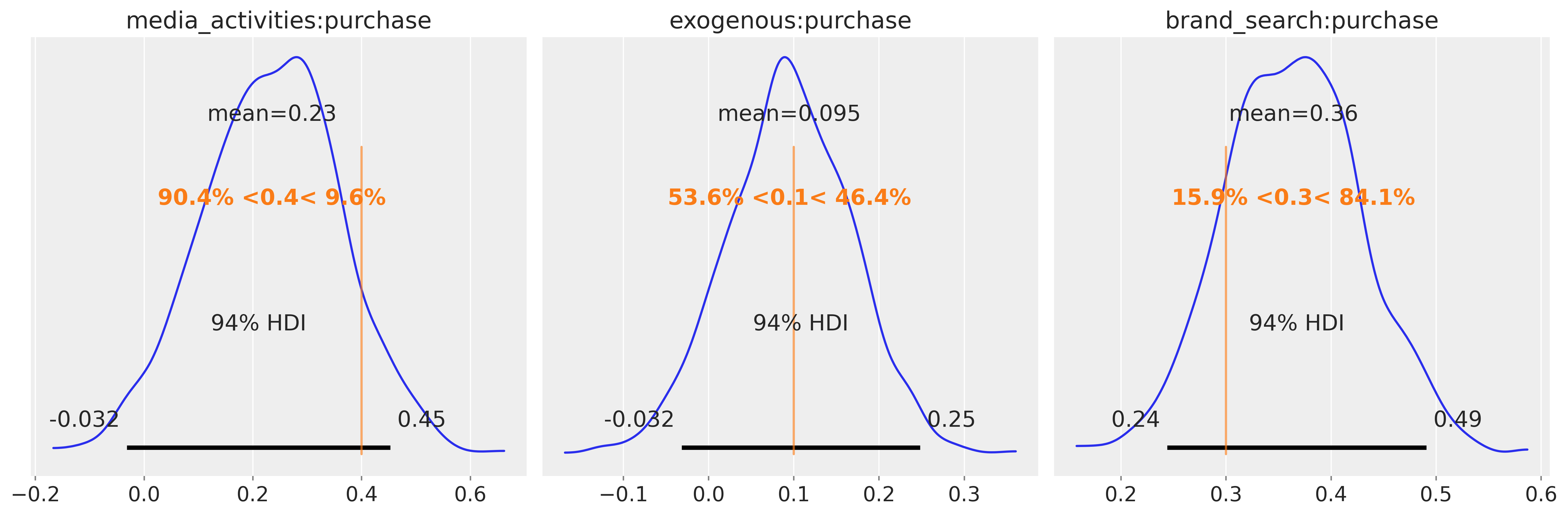
Excellent — the estimated posterior means align closely with the true underlying coefficients, confirming that our Bayesian reconstruction faithfully captured the causal signal embedded in the data.

What is particularly powerful about this approach is its simplicity: rather than building and fitting multiple regression models — one per effect or per adjustment set — we recover all estimands simultaneously within a single coherent probabilistic model. Each parameter reflects its causal interpretation directly from the DAG, and uncertainty is propagated through the full system rather than estimated piecemeal.

In this example, the graph served as the blueprint, the Bayesian model performed the joint estimation, and the result is a unified, transparent view of how each driver contributes to the outcome. This not only saves modeling effort but also ensures internal consistency — all effects are inferred together under the same causal and probabilistic assumptions.

Warning

Causal discovery caveats

All causal discovery methods rely on strong assumptions:

(i) The data-generating process is Markov and faithful to a DAG so d-separations line up with conditional independences. (ii) The measured variables capture every relevant cause (no hidden confounders) (iii) Samples are i.i.d. or at least independent enough that independence tests behave properly. (iv) The finite-sample tests are powerful enough to separate signal from noise.

The classical PC algorithm assumes causal sufficiency (no latent common causes) and acyclicity; it removes edges via conditional-independence tests and orients the remainder with Meek’s rules, so any violation of faithfulness or weak tests can leave extra or missing edges. FCI relaxes causal sufficiency by allowing latent variables and selection bias, but in return it produces a richer set of partially oriented edges (bidirected, circle endpoints) that still require strong assumptions to interpret. Because real marketing datasets often include feedback loops, non-stationarity, measurement error, and latent drivers, we treat these algorithms as hypothesis generators rather than truth oracles and bake in domain constraints wherever possible.

MMM modeling workflow

If you are thinking how this goes into the workflow to develop a model, you can visualize this as start with causal discovery, identify a credible DAG in a MEC consistent with your data, then quantify by two optional ways.

1. Causal identification route: Once the CPDAG gives you a candidate driver set for the chosen target, drop that structure into the pymc_marketing.mmm.causal model. It conditions on exactly the back-door adjustment set implied by the DAG, so you estimate each driver’s causal effect with targeted regressions or MMM variants. Great for stress-testing multiple DAGs and comparing estimands side by side.

2. Full DAG-to-model route: Feed a fully oriented DAG into BuildModelFromDAG to spin up a single PyMC model that respects the entire causal graph. Each edge gets a slope, the target retains its likelihood, and you sample the joint posterior to read off linear causal effects directly. This is ideal when you want one coherent Bayesian model rather than separate conditionals.

Warning

Soon we’ll extend BuildModelFromDAG so you can plug in nonlinear response transforms (e.g., saturation, adstock) along individual edges. That will let you stay in the DAG-driven workflow while capturing diminishing returns or channel-specific dynamics right inside the generated PyMC model.

Conclusion

Through this complete workflow — from causal discovery to Bayesian estimation — we demonstrated how structural reasoning and probabilistic modeling can be unified into a single, coherent framework.

Starting from raw data, or autocorrelated time-series data, we first learned that discovering a purely DAG is unreliable for different reasons. By introducing domain knowledge and/or explicit time-order constraints, we corrected and avoided spurious connections, allowing the graph structure to reflect true causal direction.

Once a stable DAG emerged, we transitioned from structure to substance: using BuildModelFromDAG, we converted the discovered causal relationships into a fully specified Bayesian model. This let us estimate all causal effects jointly — obtaining posterior distributions for every edge without needing to build a patchwork of separate regressions. The resulting estimands closely matched the true underlying coefficients, validating both the causal design and the Bayesian inference process.

Ultimately, this workflow illustrates the strength of an integrated causal–Bayesian approach:

• Causal discovery provides the structure (who influences whom).

• Bayesian estimation provides the magnitude (how strongly, and with what uncertainty).

Together they form a complete loop — from learning the graph, to quantifying its effects, to validating against reality.

While no method is immune to confounding or model misspecification, this pipeline offers a principled and efficient way to reason about complex systems, such as marketing data, where many drivers interact between themself and over time. It replaces fragmented analyses with a unified, interpretable, and uncertainty-aware causal model — brings meaning to our model and the ecosystem they represent.

We invite you to extend these tools—incorporate richer priors, hierarchical extensions, or dynamic components—to unlock even deeper causal insights and make more confident, data-driven decisions!

References

1. PC Algorithm for Tabular Causal Discovery

2. A fast PC algorithm for high dimensional causal discovery with multi-core PCs

3. dcFCI: Robust Causal Discovery Under Latent Confounding, Unfaithfulness, and Mixed Data

4. FCI Algorithm Introduction

%load_ext watermark
%watermark -n -u -v -iv -w -p pymc_marketing,pymc,pytensor

Last updated: Mon Oct 13 2025

Python implementation: CPython
Python version       : 3.12.11
IPython version      : 9.6.0

pymc_marketing: 0.16.0
pymc          : 5.25.1
pytensor      : 2.31.7

IPython       : 9.6.0
numpy         : 2.3.3
pandas        : 2.3.3
graphviz      : 0.21
preliz        : 0.21.0
pymc          : 5.25.1
pymc_marketing: 0.16.0
matplotlib    : 3.10.6
arviz         : 0.22.0

Watermark: 2.5.0