Understanding your MMM: Sensitivity Analysis and Marginal Effects#

Extracting insights to drive business decisions is a primary goal of any MMM. PyMC-Marketing already offers a powerful suite of tools for this, including:

Driver contributions: Understanding how much each channel or factor is contributing to the outcome.
Return on Ad Spend (ROAS): Quantifying the financial return of your media investments.
Saturation curves: Visualizing how the impact of media spend changes at different spend levels (e.g., diminishing returns).

However, in many real-world cases, we want to go beyond these summaries. Marketers and analysts frequently ask:

“What would have happened if we had spent 10% less on media last month?”
“What would the effect of lowering the free shipping threshold by $5 have been?”
“Are we still getting good incremental returns at current spend levels, or have we hit diminishing returns?”

These questions focus on hypothetical scenarios of what would have happened under different conditions. As such, they are a clear form of sensitivity analysis. Given that we focus on retrospective predictions, these questions are “Step 3” on Pearl’s causal ladder (see the MMMs and Pearl’s ladder of causal inference docs). The basic idea is that we can use our model (and what it has learned from the data) to simulate how the outcome would have changes under various peterbations of the driver variables.

Rather than just considering a single peterbation (e.g., “what if we had spent 10% less on a given media channel”), sensitivity analysis allows us to explore a range of scenarios. So instead we could evaluate our predictions given a sweep of possible peterbations. For example, “what if we had spent [0.5, 0.75, 1.0, 1.25, 2.0] times as much on a given media channel?”

We introduce a flexible tool that allows you to:

Perform counterfactual sweeps across a range of predictor values (e.g., scaling media spend up/down or adjusting business levers like pricing).
Visualize both the total expected impact of these interventions.
Compute marginal effects—showing the instantaneous rate of change in the outcome as you adjust a predictor.

This approach complements the built-in PyMC-Marketing tools by providing scenario-based insights that help you answer “what if?” questions with precision and clarity.

Setting the scene with an example dataset#

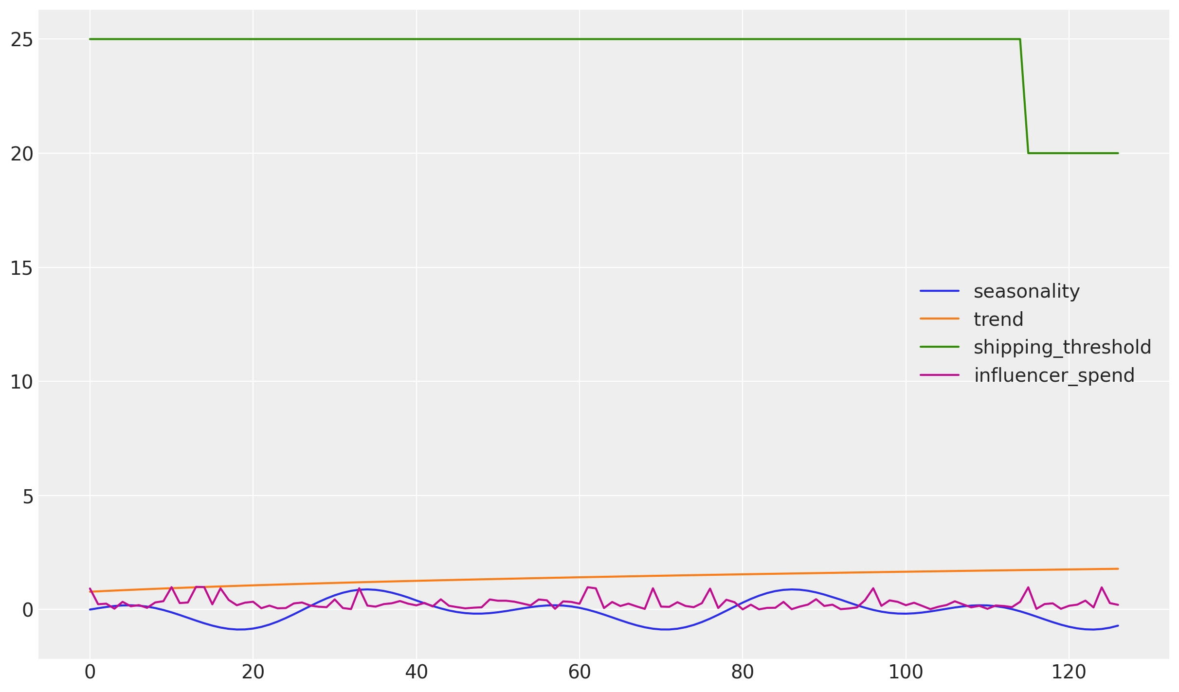
In this example, we model weekly sales for a direct-to-consumer (DTC) brand that invests in influencer marketing while also adjusting its free shipping policy to drive conversions.

Our media variable is Influencer Spend, which typically exhibits non-linear effects due to factors like audience saturation and delayed impact, making it a good candidate for adstock and saturation transformations.

As a control variable, we include the Free Shipping Threshold — the minimum order value required for customers to qualify for free shipping. This is a fully controllable business lever and is expected to have a more linear relationship with sales: lowering the threshold generally increases conversion rates in a predictable way.

By examining the marginal effects of media spend and shipping policy, we can provide actionable insights into how each lever contributes to overall performance.

import warnings

import arviz as az
import graphviz as gr
import matplotlib.pyplot as plt
import numpy as np
import pandas as pd

from pymc_marketing.mmm import (
    GeometricAdstock,
    LogisticSaturation,
)
from pymc_marketing.mmm.multidimensional import MMM
from pymc_marketing.mmm.transformers import geometric_adstock, logistic_saturation

warnings.filterwarnings("ignore", category=FutureWarning)

az.style.use("arviz-darkgrid")
plt.rcParams["figure.figsize"] = [12, 7]
plt.rcParams["figure.dpi"] = 100

%load_ext autoreload
%autoreload 2
%config InlineBackend.figure_format = "retina"

seed: int = sum(map(ord, "ladder"))
rng: np.random.Generator = np.random.default_rng(seed=seed)

OMP: Info #276: omp_set_nested routine deprecated, please use omp_set_max_active_levels instead.
/Users/carlostrujillo/Documents/GitHub/pymc-marketing/pymc_marketing/mmm/multidimensional.py:216: FutureWarning: This functionality is experimental and subject to change. If you encounter any issues or have suggestions, please raise them at: https://github.com/pymc-labs/pymc-marketing/issues/new
  warnings.warn(warning_msg, FutureWarning, stacklevel=1)

So our causal MMM will look like this:

../../_images/0e40c3bdb604bf3640c191d596292ad8c95da68d2bc51cf0a0efe61b720b120f.svg

Why Marginal Effects Matter: going beyond raw media curves#

In Media Mix Models (MMM), we’re often interested in understanding how each marketing input (like advertising spend) drives business outcomes. A common way to explore this is by looking at the inferred response curves, such as the saturation curve for media spend. These curves show how total sales respond to increasing investment, accounting for effects like diminishing returns and adstock.

But while these plots are useful, they can be misleading or incomplete when used in isolation.

The reason? Response curves tell you the absolute level of impact across different spend amounts, but they don’t directly tell you the incremental impact of a small change in spend at any given point. This distinction is crucial. For example:

A saturation curve might look steep at low spend levels and flatten out at higher spend—but the exact slope at a specific point (e.g., $50,000 per week) tells you the real-world payoff of spending an extra $1,000 right now.
In cases where multiple inputs are at play (like media spend and pricing changes), response curves for one variable don’t show you how interactions or current levels of other variables might affect its marginal impact.

Marginal effects zero in on this slope—the instantaneous rate of change. They answer questions like:

How much additional sales do I gain if I increase influencer spend by 10% next week?
What’s the expected lift if I lower the free shipping threshold by $5 right now?

These insights are only accessible through marginal effects because they reflect the dynamic, context-sensitive responsiveness of the model:

For media inputs with non-linear transformations (like adstock + saturation), marginal effects show how effectiveness varies across the spend range—revealing whether you’re still in the high-ROI zone or have hit diminishing returns.
For controllable non-media levers (like pricing or shipping policies), marginal effects provide precise, actionable estimates for how tweaks to these levers impact outcomes—even if their overall relationship is more linear.

In other words, while a response curve is like a map of the terrain, marginal effects tell you whether it’s worth climbing that next hill. They enable surgical precision in decision-making, ensuring that marketers don’t just see where their efforts sit on a curve—but understand whether pushing harder in a particular direction is still worthwhile.

By incorporating marginal effects into MMM outputs, we move from a static understanding of media performance to a dynamic, context-aware view that directly informs resource allocation and strategic adjustments.

Generate simulated data#

Show code cell source

Hide code cell source

def apply_transformations(df, channel, alpha, lam):
    """Apply geometric adstock and saturation transformations."""
    adstocked = geometric_adstock(
        x=df[channel].to_numpy(), alpha=alpha, l_max=8, normalize=True
    ).eval()

    saturated = logistic_saturation(x=adstocked, lam=lam).eval()
    return saturated


def forward_pass(df_in, params):
    """Run predictor variables through the forward pass of the model.

    Given a dataframe with spend data columns and control variables, run this through the
    transformations and return the response variable `y`.
    """
    df = df_in.copy()

    # Apply transformations to channels and calculate y
    df["y"] = params["amplitude"] * (
        df["intercept"]
        + df["trend"]
        + df["seasonality"]
        + sum(
            params["beta"][i]
            * apply_transformations(
                df, params["channels"][i], params["alpha"][i], params["lam"][i]
            )
            for i in range(len(params["channels"]))
        )
        + params["gamma"] * df["shipping_threshold"]  # Include shipping_threshold
        + df["epsilon"]
    )

    return df


df = pd.DataFrame(
    data={
        "date": pd.date_range(
            start=pd.to_datetime("2019-04-01"),
            end=pd.to_datetime("2021-09-01"),
            freq="W-MON",
        )
    }
).assign(
    year=lambda x: x["date"].dt.year,
    month=lambda x: x["date"].dt.month,
    dayofyear=lambda x: x["date"].dt.dayofyear,
    t=lambda x: range(x.shape[0]),
)

n_rows = df.shape[0]

# Media data: influencer spend
influencer_spend = rng.uniform(low=0.0, high=1.0, size=n_rows)
df["influencer_spend"] = np.where(
    influencer_spend > 0.9, influencer_spend, influencer_spend / 2
)

# Control variable: shipping threshold
df["shipping_threshold"] = 25.0
df.loc[df.index[-12:], "shipping_threshold"] = (
    20.0  # Reduced shipping threshold in the last 12 weeks
)
# Intercept, trend, seasonality components
df["intercept"] = 2.0
df["trend"] = (np.linspace(start=0.0, stop=50, num=n_rows) + 10) ** (1 / 4) - 1
df["cs"] = -np.sin(2 * 2 * np.pi * df["dayofyear"] / 365.5)
df["cc"] = np.cos(1 * 2 * np.pi * df["dayofyear"] / 365.5)
df["seasonality"] = 0.5 * (df["cs"] + df["cc"])

# Noise - can be considered as the effects of unobserved variables upon sales
df["epsilon"] = rng.normal(loc=0.0, scale=0.25, size=n_rows)

params = {
    "channels": ["influencer_spend"],
    "amplitude": 1.0,
    "beta": [3.0],
    "lam": [4.0],
    "alpha": [0.4],
    "gamma": -0.1,  # Weight for shipping_threshold
}

df = forward_pass(df, params)

And here are the first 5 rows of the synthetic dataset:

df.head()

	date	year	month	dayofyear	t	influencer_spend	shipping_threshold	intercept	trend	cs	cc	seasonality	epsilon	y
0	2019-04-01	2019	4	91	0	0.918883	25.0	2.0	0.778279	-0.012893	0.006446	-0.003223	-0.118826	2.561363
1	2019-04-08	2019	4	98	1	0.230898	25.0	2.0	0.795664	0.225812	-0.113642	0.056085	0.064977	2.264874
2	2019-04-15	2019	4	105	2	0.254486	25.0	2.0	0.812559	0.451500	-0.232087	0.109706	-0.020269	1.998208
3	2019-04-22	2019	4	112	3	0.035995	25.0	2.0	0.828993	0.651162	-0.347175	0.151993	0.400209	1.701116
4	2019-04-29	2019	4	119	4	0.336013	25.0	2.0	0.844997	0.813290	-0.457242	0.178024	0.057609	2.003646

And we can plot the data to get a better sense for the data:

df[["seasonality", "trend", "shipping_threshold", "influencer_spend"]].plot();

../../_images/dd891fcfa49701fc1526f78dada16f8ff62c4d96b02d291c796e22b7c40da897.png

Build and fit the MMM#

mmm = MMM(
    date_column="date",
    target_column="y",
    adstock=GeometricAdstock(l_max=8),
    saturation=LogisticSaturation(),
    channel_columns=["influencer_spend"],
    control_columns=["t", "shipping_threshold"],
    yearly_seasonality=2,
)

x_train = df.drop(columns=["y"])
y_train = df["y"]

mmm.fit(
    X=x_train,
    y=y_train,
)
mmm.sample_posterior_predictive(x_train, extend_idata=True);

Sensitivity analysis and marginal effects#

A multiplicative sweep on influencer spend#

sweeps = np.linspace(0.1, 2.0, 100)

mmm.model.to_graphviz()

../../_images/5836fdefb5721003415bba95046ef24a5a190cac2523058bb33e38449de3dc2e.svg

Influencer spend exist under channel_* nodes. In our graph, every individual driver will exist under those containers. We could calculate a sweep over any variable (node) in the computational graph, in this case, we pick channel data to be able to access later on influencer_spend.

Note: This compute deterministic not using aleatoric uncertainty from likelihood. Meaning, the sigma parameter for the likelihood will not modify our sweep.

mmm.sensitivity.run_sweep(
    sweep_values=sweeps,
    var_input="channel_data",
    var_names="channel_contribution",
    extend_idata=True,
);

The code above saves its results into a new group in the mmm.idata called sensitivity_analysis. You can explore it below:

mmm.idata

arviz.InferenceData

Tip

The group sensitivity analysis contains all the channels from the node channel_contribution. Meaning, you can select whatever channel you want.

And of course, you can plot the results! To demonstrate some of the plotting options we’ll plot using the default y-axis scale of absolute sales.

_ = mmm.plot.sensitivity_analysis(
    aggregation={"sum": ("channel",)},
    xlabel="Sweep multiplicative",
    ylabel="Total contribution over training period",
);

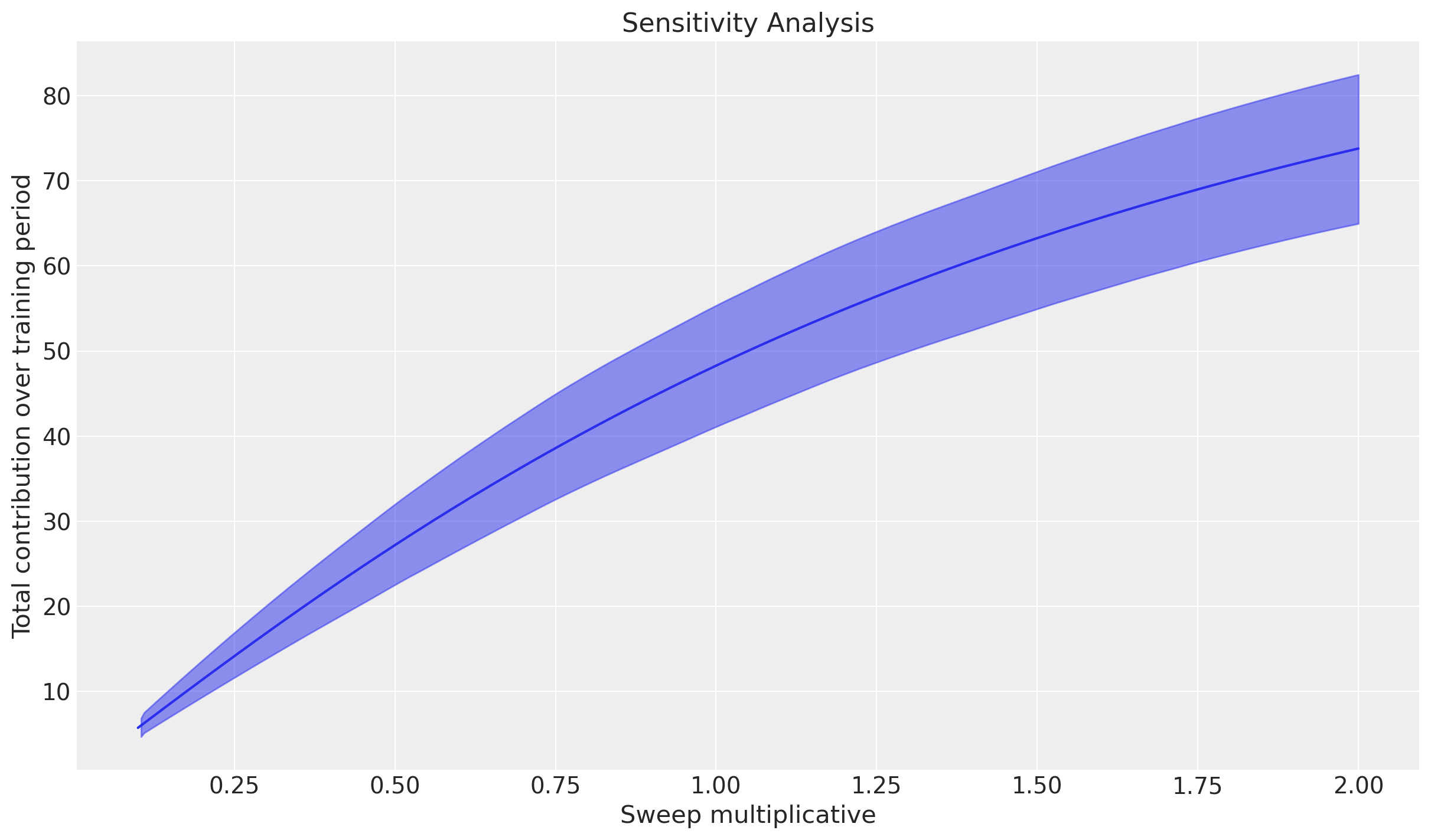
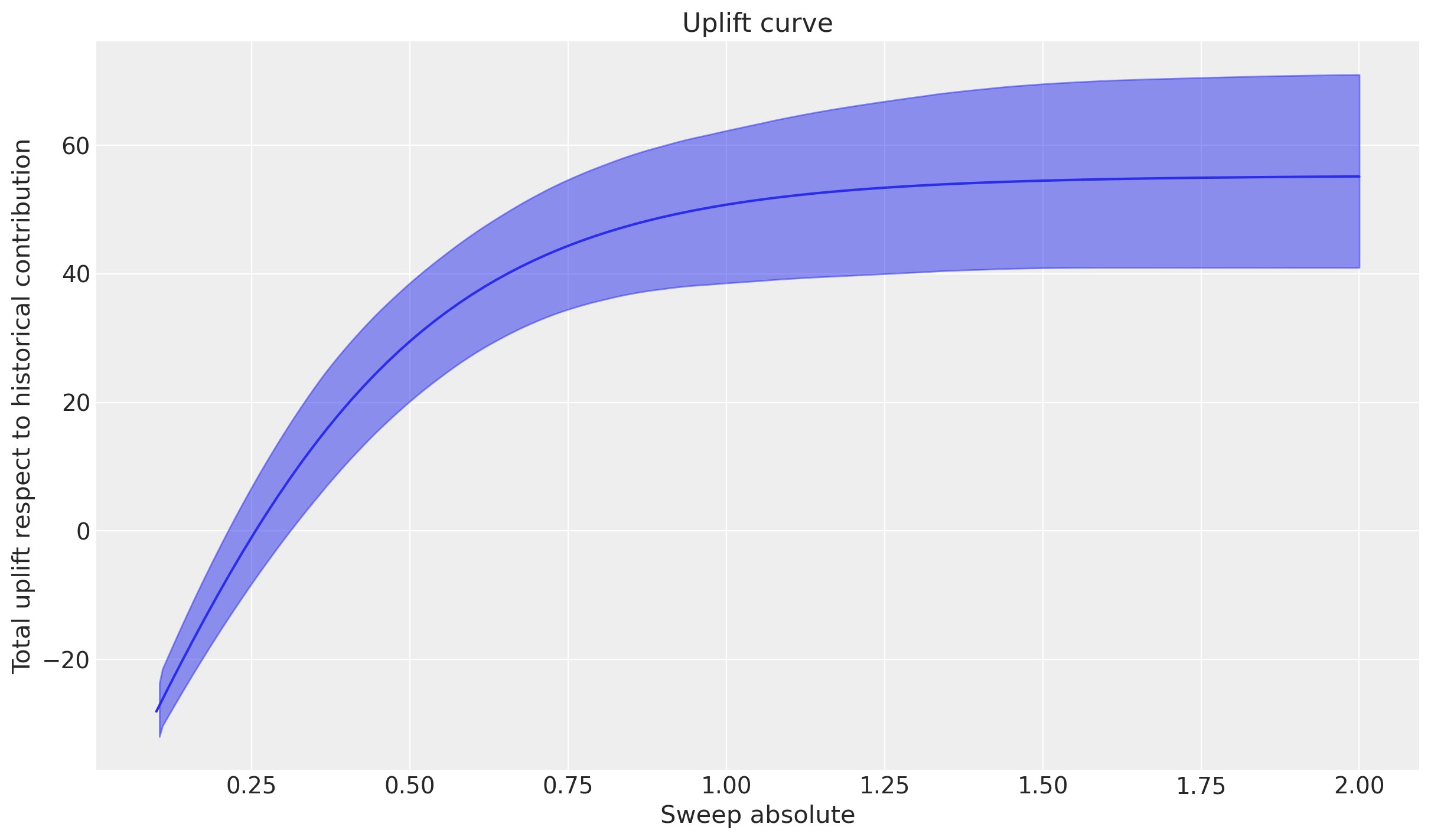
../../_images/4f2737ab50327eb6021ee0d0f66249a65459643bc6893e2d6427cf3a9d507433.png

We did a multiplicative sweep. X will be the multiplicative factor and Y the total incremental conversions during the full training period at the given multiplicative factor. We could visualize this as certain uplift, respect to an arbitrary number.

For this case, we can use the historical contributions as our reference point. This will generate a curve that shows the relative uplift when we increase or decrease spending. For example: if we maintain the same spending level, the uplift relative to the current contribution will be zero. However, if we increase spending, we’ll see a positive uplift, and conversely, if we decrease spending, we’ll observe a negative uplift.

ref_value = (
    mmm.idata.posterior.channel_contribution.sum(
        ["channel", "date"]
    )  # The ref can be your spend level during training
    .mean(["chain", "draw"])
    .item()
)

mmm.sensitivity.compute_uplift_curve_respect_to_base(
    results=mmm.idata.sensitivity_analysis["x"],
    ref=ref_value,
    extend_idata=True,
);

_ = mmm.plot.uplift_curve(
    aggregation={"sum": ("channel",)},
    xlabel="Sweep multiplicative",
    ylabel="Total uplift respect to historical contribution",
)
# add vertical line at zero
plt.axvline(x=1.0, color="black", linestyle="--")
# add horizontal line at zero
plt.axhline(y=0.0, color="black", linestyle="--");

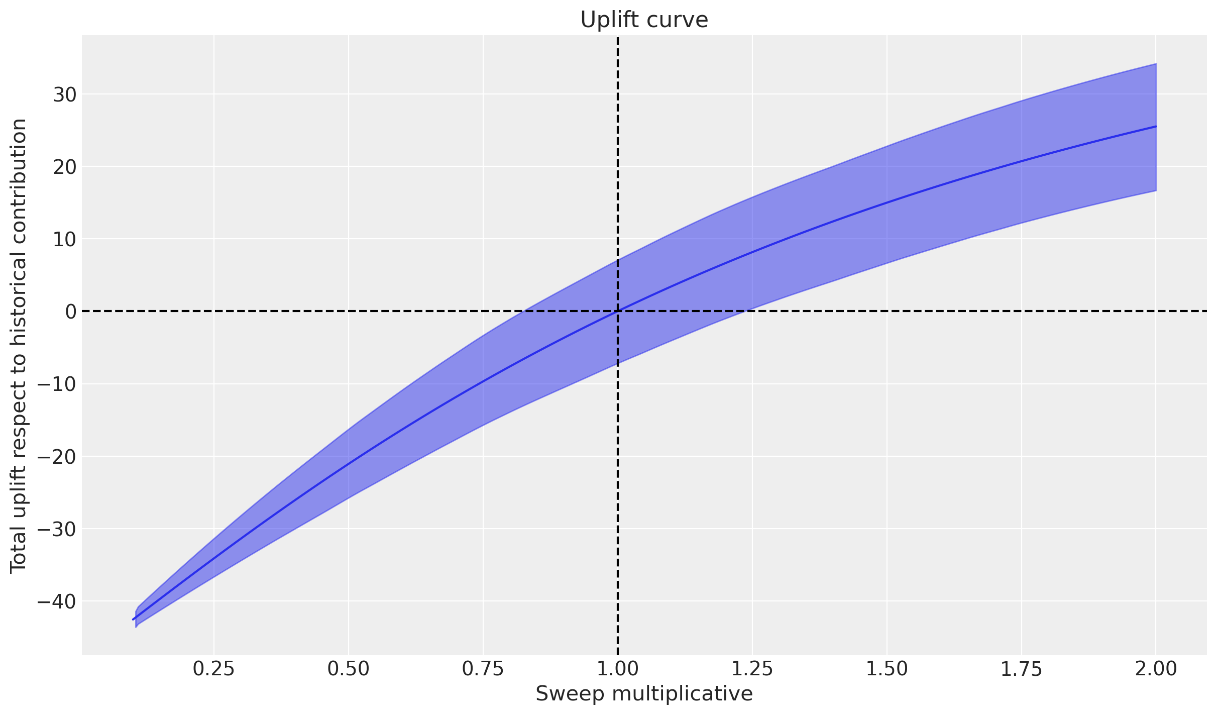
../../_images/58c65ff52608a27aa49e72fd60ee48a9e0404cca9c866918777e2b94cb05032e.png

The figure above shows the total expected uplift (it can be positive or negative) for the outcome variable as a function of the sweep values provided. In this case, we used a multiplicative sweep, so the curve is showing how the total outcome would vary if we multiply up (sweep values > 1) or down (sweep values < 1) the influencer spend by the set of values we asked for.

Intuitively, if we multiply the influence spend by 1.0 then on average we expect no change. If we scale the spend down then we expect negative uplift (i.e., lower sales) and if we scale the spend up then we expect positive uplift (i.e., higher sales). The fact that the curve is curved (not linear) is primarily the result of the saturation function on the influencer spend variable.

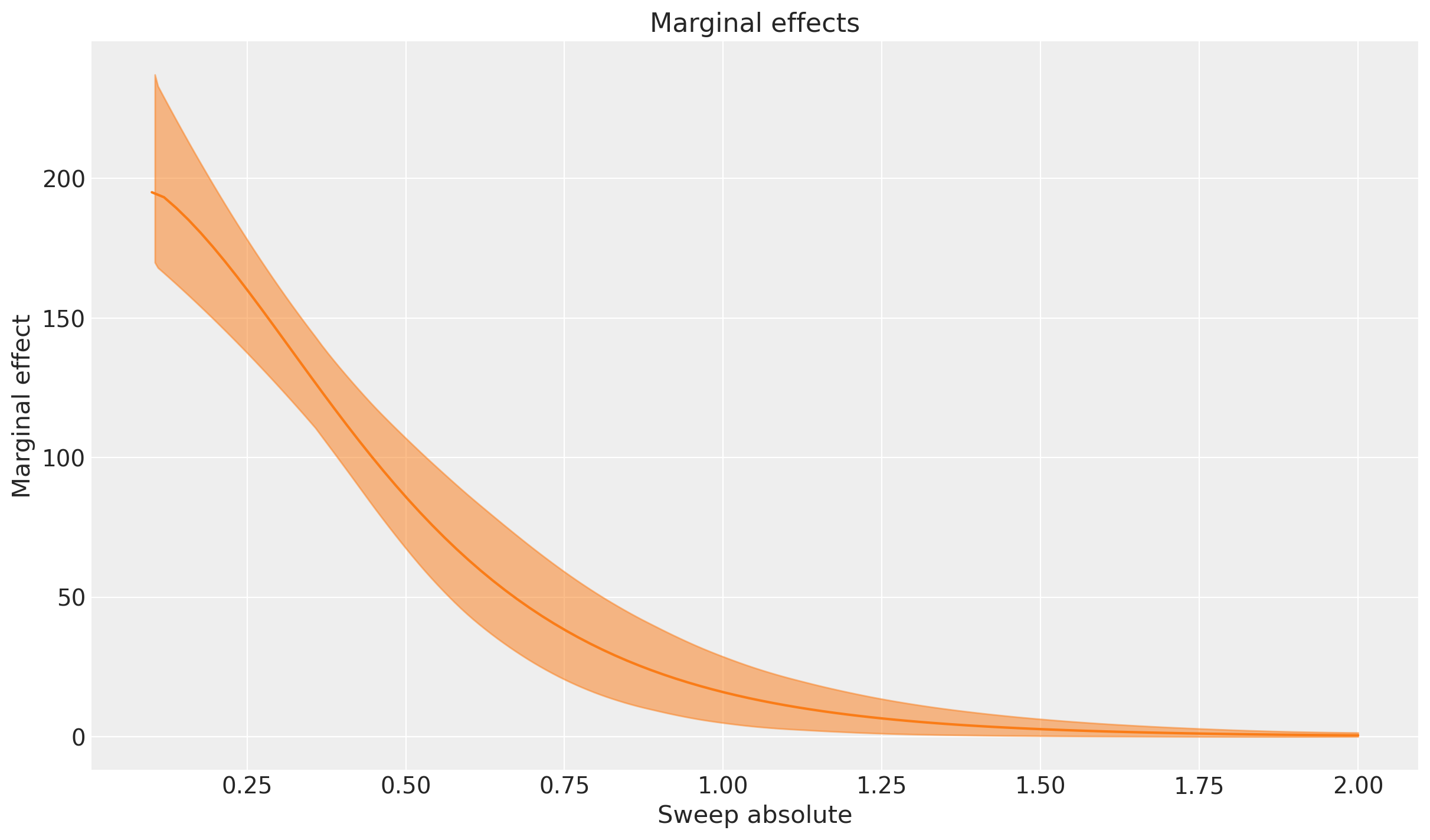
We can also plot the corresponding marginal effects from the uplift curve as below:

mmm.sensitivity.compute_marginal_effects(
    results=mmm.idata.sensitivity_analysis["uplift_curve"], extend_idata=True
);

_ = mmm.plot.marginal_curve(
    aggregation={"sum": ("channel",)}, xlabel="Sweep multiplicative"
);

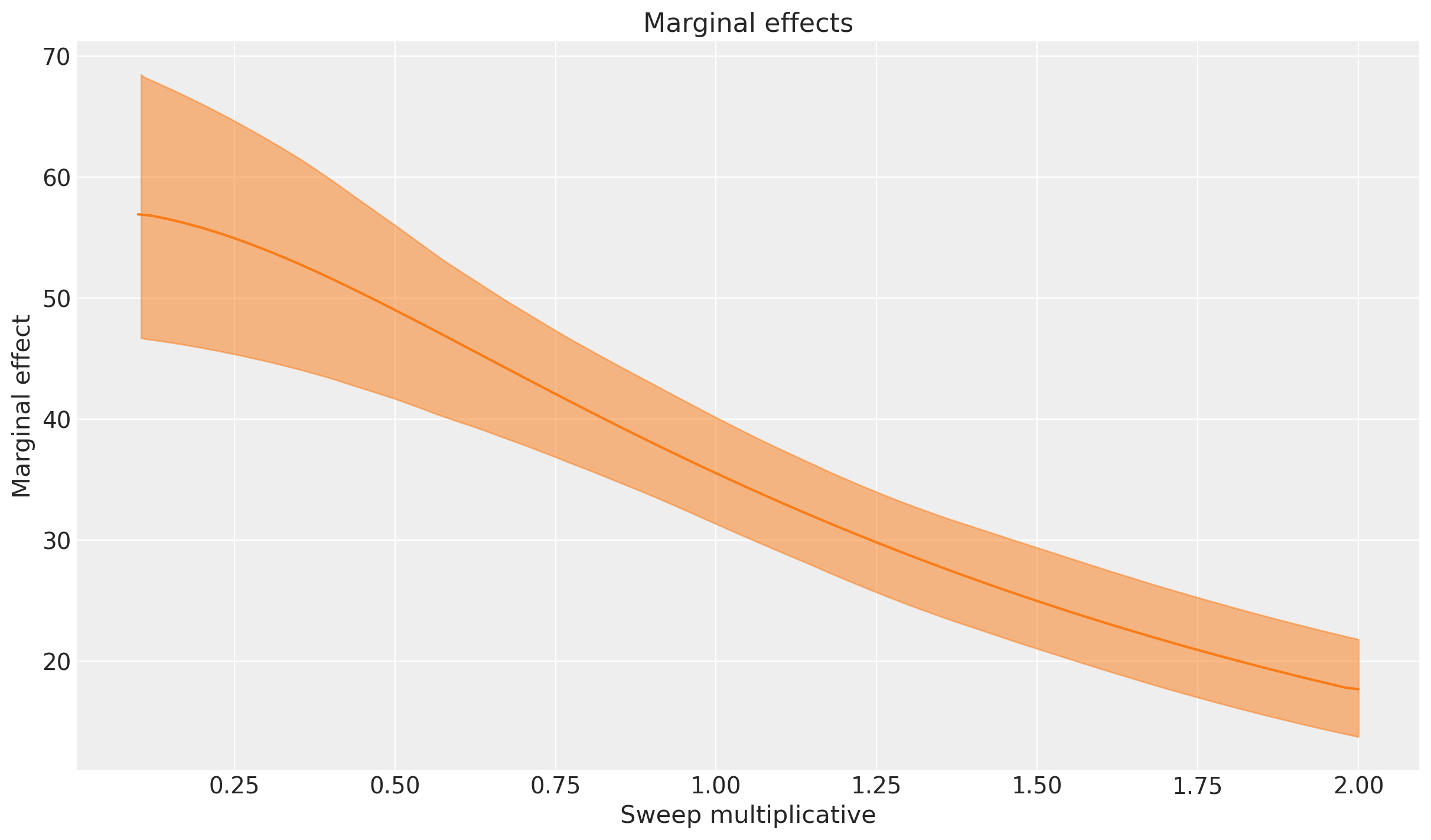
../../_images/dfdd195d718d9fc290aa038257ded51fea3aebcbc7d1554a377bbb22b90f6d1b.png

This plot shows the instantaneous rate of change in the outcome variable as we adjust the influencer spend. The y-axis represents the marginal effect, which tells us how much additional sales we expect for a small increase in influencer spend at each point along the sweep values.

We can see that the highest marginal effects occur on the left side of the plot where we the influence spend is zero or very low. The highest incremental/marginal effects are obtained when we go from no spend to some spend. As we would expect from the previous plot, we still get incremental returns at the current spend levels (multiplicative change of 1.0), and are quite far away from totally saturating this channel - the marginal spend doesn’t reduce to near zero even if we consider a 2x increase in spend.

An absolute sweep on influencer spend#

The sensitivity analysis we conducted above involved a multiplicative sweep of the influencer spend variable, meaning we varied it by multiplying it by a set of values. However, we can also conduct a absolute sweep. Here, we set all historical values of the influencer spend variable to fixed values (given in the sweep_values argument) and then compute the expected outcome and marginal effects.

mmm.sensitivity.run_sweep(
    sweep_values=sweeps,
    var_input="channel_data",
    var_names="channel_contribution",
    sweep_type="absolute",
    extend_idata=True,
);

ref_value = (
    mmm.idata.posterior.channel_contribution.sum(["channel", "date"])
    .mean(["chain", "draw"])
    .item()
)
mmm.sensitivity.compute_uplift_curve_respect_to_base(
    results=mmm.idata.sensitivity_analysis["x"],
    ref=ref_value,
    extend_idata=True,
)

mmm.sensitivity.compute_marginal_effects(
    results=mmm.idata.sensitivity_analysis["uplift_curve"], extend_idata=True
)

_ = mmm.plot.uplift_curve(
    aggregation={"sum": ("channel",)},
    xlabel="Sweep absolute",
    ylabel="Total uplift respect to historical contribution",
)
_ = mmm.plot.marginal_curve(aggregation={"sum": ("channel",)}, xlabel="Sweep absolute");

../../_images/5625611dbbf6a65367597c6d61cf9b51a5ea5566082f43f829b91a3641722d3e.png

../../_images/1fbeebda81520fefb136bb254ad6ed439660f6726b6c1cbc3bf16ce7239549c3.png

The results of the absolute sweep are comparable to (but not the same as) the multiplicative sweep. They key difference in what we are doing is that we overwrite the historical influencer spend values with a constant spend value (one value for each point in the sweep). This means we are not considering a ‘realistic’ scenario where spend fluctuates over time, but rather a hypothetical scenario where we set the spend to a fixed value for all weeks in the dataset.

We can see the change in the plots as well. The top plot is similar to, but not exactly the same as the saturation curve of influencer spend. Notice that there is a certain fixed spend level where the uplift is about zero. This is interesting - we can interpret this as saying that the total sales in the actual scenario would also have been about the same if we had spent that amount (constantly over time) on influencer marketing.

The top plot nicely shows the saturating quality of the saturation function, and the bottom plot shows that as we approach saturation, the marginal effects drop to near zero.

An additive sweep on influencer spend#

We can also consider a sweep of additive changes to the influencer spend variable. This means we adjust the historical values of the influencer spend by adding a fixed amount (given in the sweep_values argument) and then compute the expected outcome and marginal effects.

Warning

Note that care needs to be taken with an additive sweep. It would be easy to apply a negative peterbation which then actually results in negative spend values which have no meaningful interpretation. So it is worthwhile exploring the actual spend values before deciding on the sweep values to be used.

In our case, the minimum spend values is $0, so we will not considervalues in the sweep.

df["influencer_spend"].min()

../../_images/3b80ecf7b88045171178e6218bce9bb50b647cc5d8e2f716e6a51dabc2fc0401.png

mmm.sensitivity.run_sweep(
    sweep_values=sweeps,
    var_input="channel_data",
    var_names="channel_contribution",
    sweep_type="additive",
    posterior_sample_fraction=0.98,
    extend_idata=True,
);

Tip

The posterior_sample_fraction parameter cuts your posterior, reducing the computational burden in the process. If you have large models, this can help you to compute your sweep more efficiently because you don’t need the full posterior to get the estimate. A random subsmaple of the posterior should be enough if your posterior has not longer tails or skewness.

ref_value = (
    mmm.idata.posterior.channel_contribution.sum(["channel", "date"])
    .mean(["chain", "draw"])
    .item()
)
mmm.sensitivity.compute_uplift_curve_respect_to_base(
    results=mmm.idata.sensitivity_analysis["x"],
    ref=ref_value,
    extend_idata=True,
)

mmm.sensitivity.compute_marginal_effects(
    results=mmm.idata.sensitivity_analysis["uplift_curve"], extend_idata=True
)

_ = mmm.plot.uplift_curve(
    aggregation={"sum": ("channel",)},
    xlabel="Sweep additive",
    ylabel="Total uplift respect to historical contribution",
)
_ = mmm.plot.marginal_curve(aggregation={"sum": ("channel",)}, xlabel="Sweep additive");

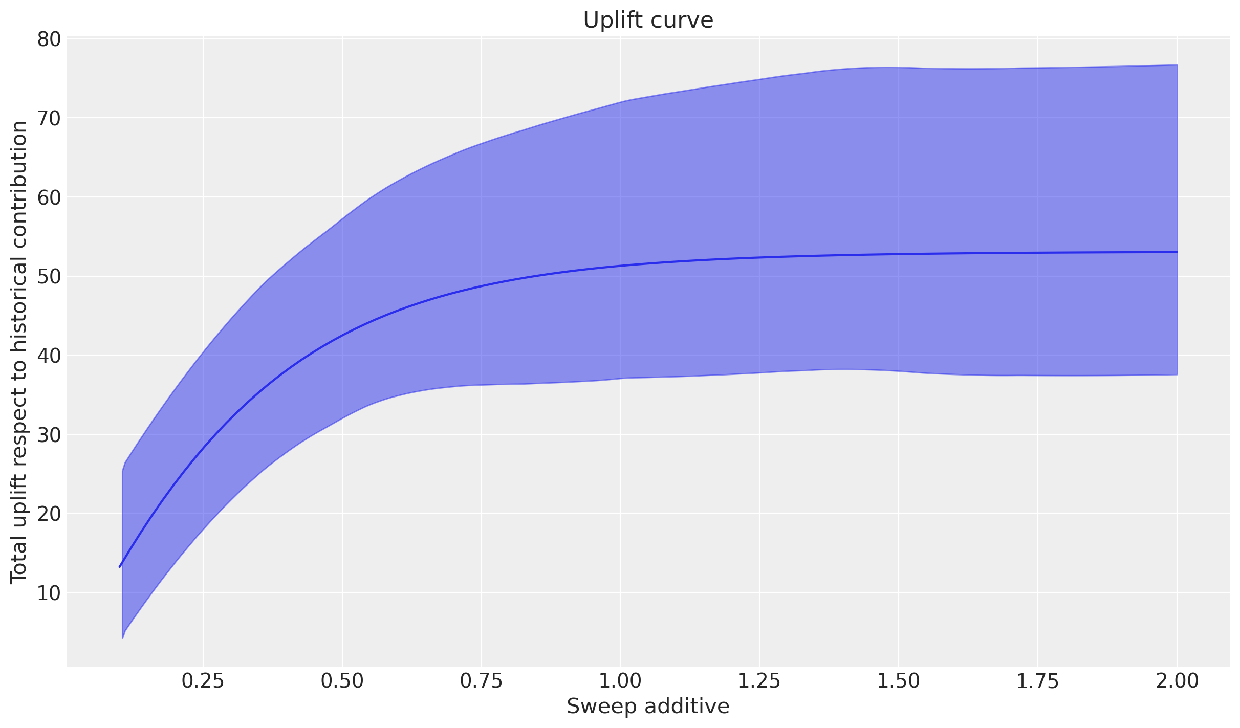
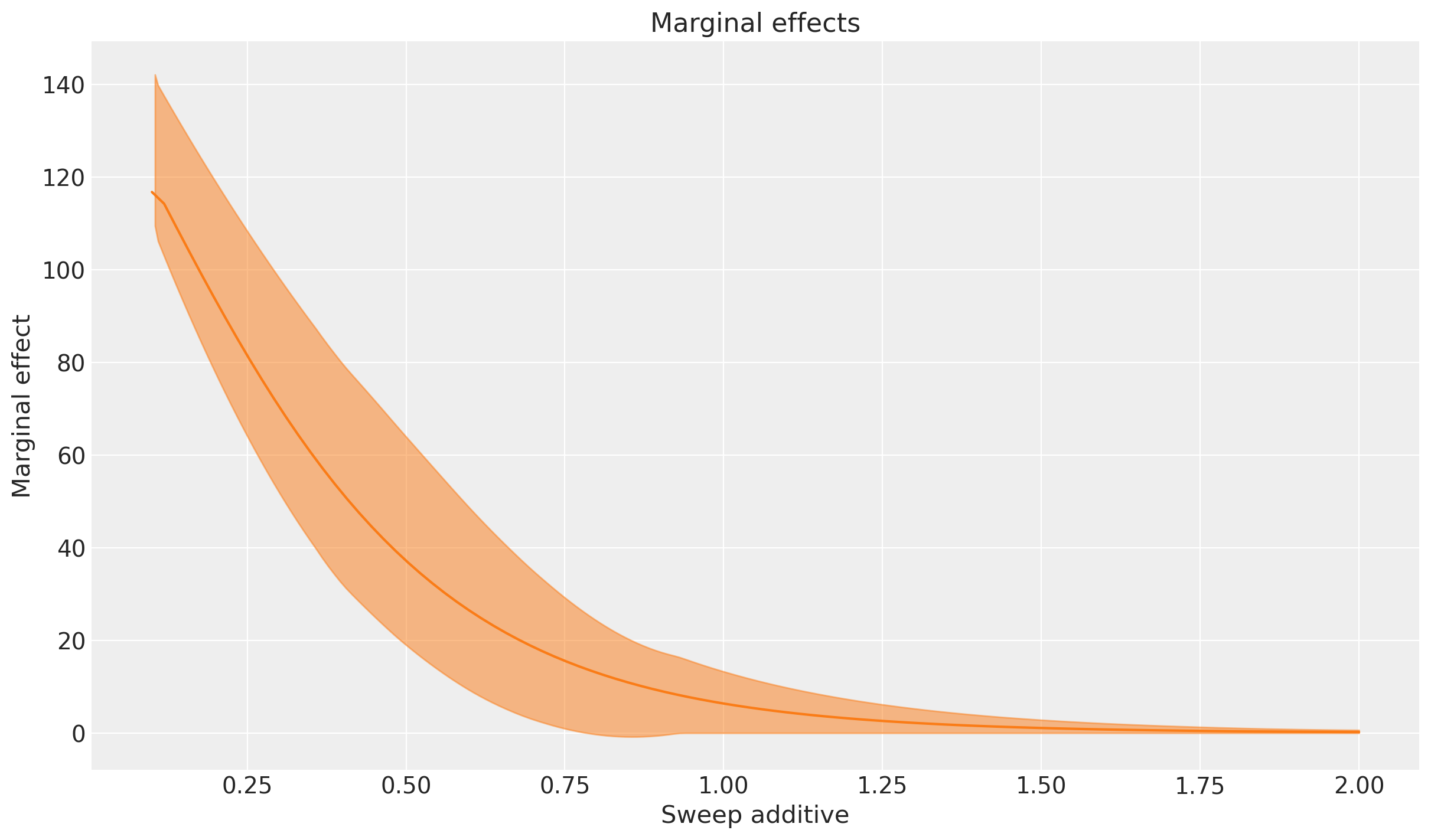
../../_images/c3dad63ffb287f7abb1327cd308063170b0e977c6b0ae9aa61b831a732d38b85.png

../../_images/b77a4619b1d83860bf0bae158bcd67f005d6ddc8a8baf86156416277c0f71d8a.png

These plots show the expected uplift and marginal effects. We get a similar general pattern of results - if we consider scenarios where we had spent progressively more, then we would get positive uplift, but as we reach a certain level of spend, the advertising channel saturates and the marginal effects drop to near zero.

Sensitivity analysis on the free shipping threshold#

We’ve had a thorough look at the influencer spend variable and we’ve got some interesting insights into how it affects the outcome (sales) under different counterfactual scenarios.

But we can also do the same for the free shipping threshold driver. The reason why this is interesting in our example is because this driver is assumed to have linear effects on the outcome, with no saturation or adstock function applied.

We won’t exhaustively run through all the different sweeps we can do, but we will just demonstrate an absolute sweep.

mmm.sensitivity.run_sweep(
    sweep_values=sweeps,
    var_input="control_data",
    var_names="control_contribution",
    sweep_type="absolute",
    extend_idata=True,
);

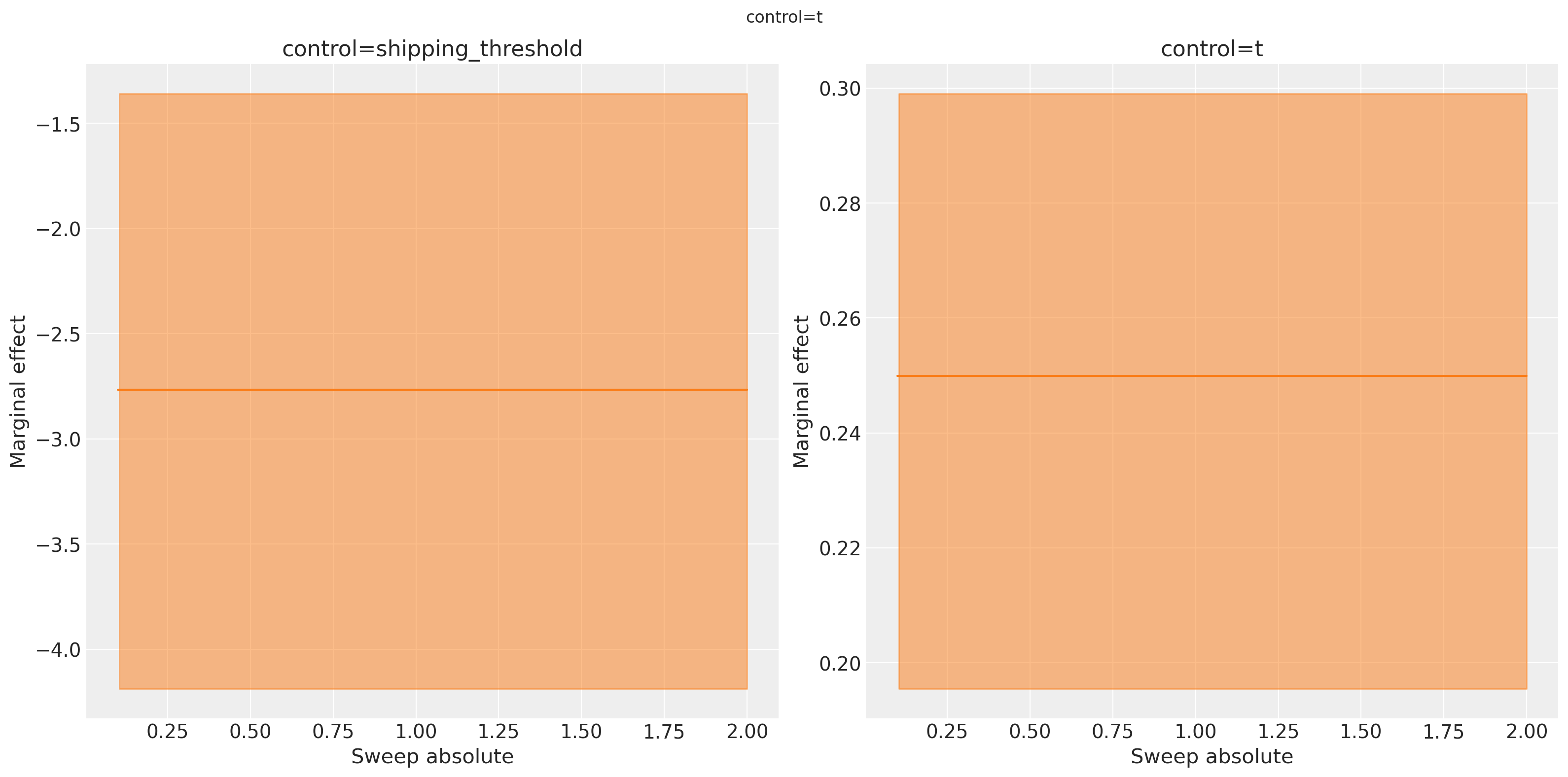
Because we make the sweep for all variables in the control contribution container, then we can plot actually all of them automatically. In this case, we have trend and shipping_threshold.

ref_value = mmm.idata.posterior.control_contribution.sum(["date"]).mean(
    ["chain", "draw"]
)
mmm.sensitivity.compute_uplift_curve_respect_to_base(
    results=mmm.idata.sensitivity_analysis["x"],
    ref=ref_value,
    extend_idata=True,
)

mmm.sensitivity.compute_marginal_effects(
    results=mmm.idata.sensitivity_analysis["uplift_curve"], extend_idata=True
)

_ = mmm.plot.uplift_curve(
    subplot_kwargs={"figsize": (16, 8)},
    xlabel="Sweep absolute",
    ylabel="Total uplift respect to historical contribution",
)
_ = mmm.plot.marginal_curve(
    subplot_kwargs={"figsize": (16, 8)}, xlabel="Sweep absolute"
);

/Users/carlostrujillo/Documents/GitHub/pymc-marketing/pymc_marketing/mmm/plot.py:1717: UserWarning: The figure layout has changed to tight
  fig.tight_layout()
/Users/carlostrujillo/Documents/GitHub/pymc-marketing/pymc_marketing/mmm/plot.py:1717: UserWarning: The figure layout has changed to tight
  fig.tight_layout()

../../_images/6b4f574de32c4a5674546afbb51d9b3850f6ea1625efd2436d4f868d996f5db1.png

../../_images/7a867eca47e460a0fa5eea9e40682855e1cdcd52a958f9733287f70b81c6b632.png

We can select only one and plot as well if thats what we want.

ref_value = (
    mmm.idata.posterior.control_contribution.sel(control="shipping_threshold")
    .sum(["date"])
    .mean(["chain", "draw"])
)
mmm.sensitivity.compute_uplift_curve_respect_to_base(
    results=mmm.idata.sensitivity_analysis["x"].sel(control="shipping_threshold"),
    ref=ref_value,
    extend_idata=True,
)

mmm.sensitivity.compute_marginal_effects(
    results=mmm.idata.sensitivity_analysis["uplift_curve"], extend_idata=True
)

_ = mmm.plot.uplift_curve(
    subplot_kwargs={"figsize": (16, 8)},
    xlabel="Sweep absolute",
    ylabel="Total uplift respect to historical contribution",
)
_ = mmm.plot.marginal_curve(
    subplot_kwargs={"figsize": (16, 8)}, xlabel="Sweep absolute"
);

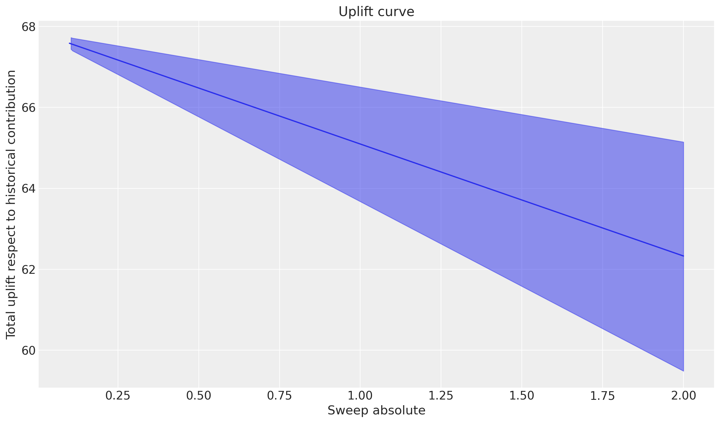
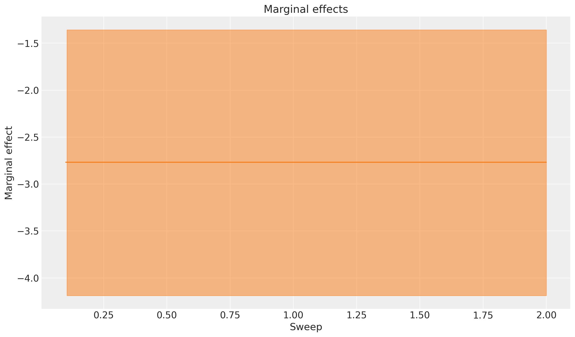
../../_images/647fc002985baf8f52bf600facf3a42cf99300d06c4b144296f98cd45ce49940.png

../../_images/e7f6ac0478eacfa04f1fd3f1acb92de52f2ea59b11476a1dd41a97f1aca0d070.png

We can see the linear nature of the effects of the free shipping threshold on the outcome variable. The expected uplift is positive when we lower the threshold (people buy more when shipping is free), and the marginal effects are constant across the sweep values. This is because we assumed a linear relationship between the free shipping threshold and sales, so the marginal effect does not change as we adjust the threshold. The constant negative value is equal to the change in uplift as we increase the shipping threshold by $1.

We can verify this by changing the sweep step size and seeing that we get identical marginal effects estimates (albeit with numerical estimation error).

mmm.sensitivity.run_sweep(
    sweep_values=sweeps,
    var_input="control_data",
    var_names="control_contribution",
    sweep_type="absolute",
    extend_idata=True,
);

ref_value = (
    mmm.idata.posterior.control_contribution.sel(control="shipping_threshold")
    .sum(["date"])
    .mean(["chain", "draw"])
    .item()
)
mmm.sensitivity.compute_uplift_curve_respect_to_base(
    results=mmm.idata.sensitivity_analysis["x"].sel(control="shipping_threshold"),
    ref=ref_value,
    extend_idata=True,
)

mmm.sensitivity.compute_marginal_effects(
    results=mmm.idata.sensitivity_analysis["uplift_curve"], extend_idata=True
)

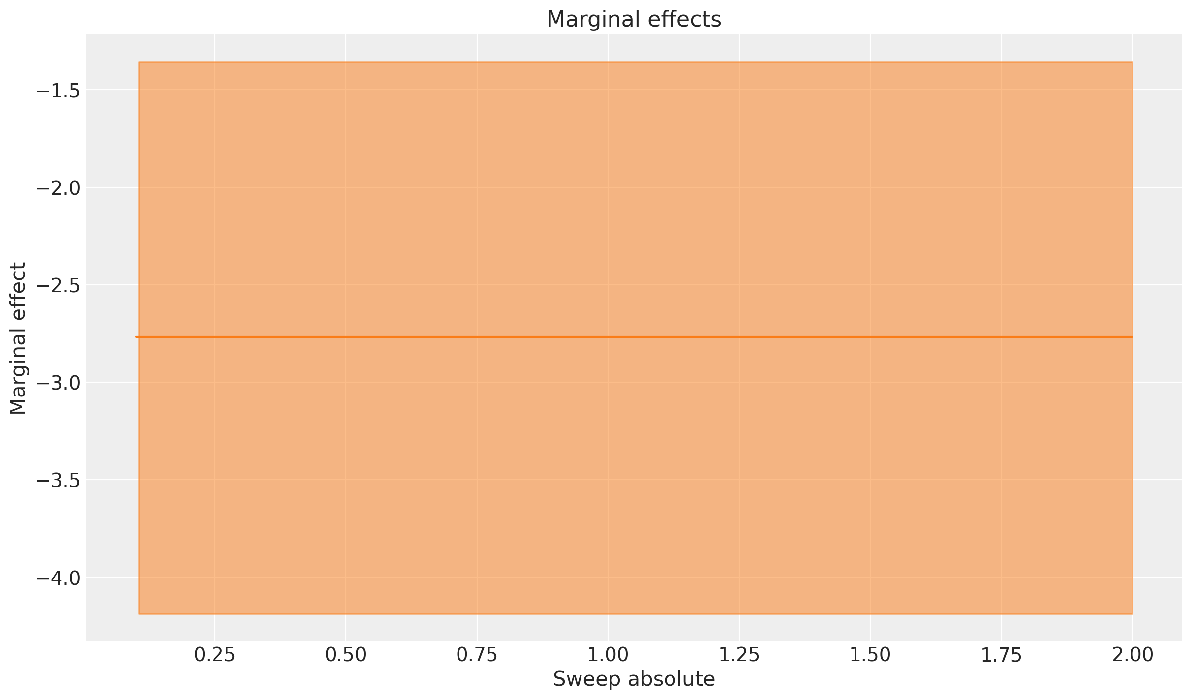
_ = mmm.plot.uplift_curve(aggregation={"sum": ("channel",)})
_ = mmm.plot.marginal_curve(aggregation={"sum": ("channel",)});

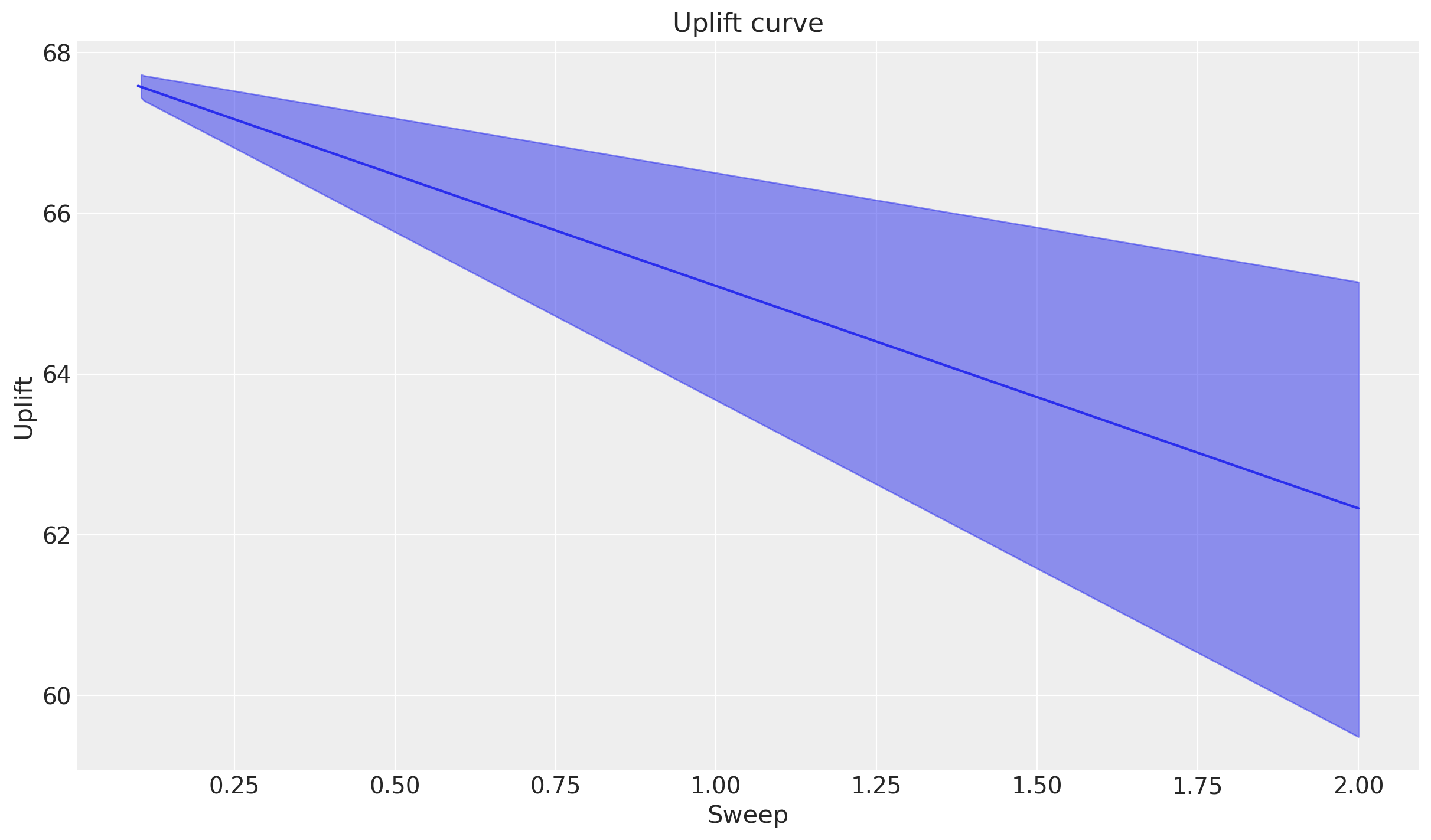
../../_images/07a812cb69722ed41a71f90de46953a44905c87e2e1f096c63665fe96d8a8cc0.png

../../_images/d573d1a0b33cdf2c3b4bb4bf24d2593c3f9895c3c0f165147487447d071d0908.png

Tip

Why should I be interested in a straight line and a flat line? These are the kinds of plots that you can run through to get a sense check of whether the model is behaving as expected.

Maybe you (or a client) realises that a negative linear relationship between shipping threshold and sales is too simplistic. This can then drive model iteration and improvement - you could explore alternative functional forms for example.

Summary#

We’ve introduced a simple but powerful tool for probing deeper into your MMM results. You can explore a sweep of perterbations to one or more driver variables and compute the expected outcomes and marginal effects for each scenario. You can consider different forms of peterbation, here we’ve shown multiplicative, absolute and additive sweeps.

This allows you to answer “what if” questions with precision and clarity, providing actionable insights into how different levers affect your business outcomes. You can produce simple and interpretable plots that you can use to communicate how the model works and get sense-checks on the model’s behaviour and assumptions.

%load_ext watermark
%watermark -n -u -v -iv -w -p pymc_marketing,pytensor

Last updated: Mon Oct 27 2025

Python implementation: CPython
Python version       : 3.12.11
IPython version      : 9.6.0

pymc_marketing: 0.16.0
pytensor      : 2.31.7

pymc_marketing: 0.16.0
graphviz      : 0.21
arviz         : 0.22.0
matplotlib    : 3.10.6
numpy         : 2.3.3
pandas        : 2.3.3

Watermark: 2.5.0